Fidelity in LLM Information Processing

In audio engineering, fidelity measures how faithfully a system reproduces its input signal. A high-fidelity amplifier preserves the source recording; a low-fidelity one introduces distortion, clips peaks, and loses detail. The same concept applies whenever information passes through a processing chain -- including the chains we build with large language models.

Executive Summary

• Summarization is lossy compression with three predictable failure modes: numerical precision loss, attribution erasure, and conditional nuance collapse.
• Multi-hop pipelines compound errors -- fidelity degrades exponentially with each step unless the system re-consults the source.
• Token budgets are bandwidth. Stuffing a context window past the point of useful information degrades output quality, not improves it.
• Five strategies preserve fidelity: structured source attribution, hierarchical summarization, chain-of-thought transparency, retrieval over compression, and explicit preservation contracts.
• Fidelity measurement is asymmetric -- detecting hallucinated additions is easier than detecting critical omissions. Recall-oriented checks require defining what "critical" means up front.
• Larger context windows shift the problem from "what fits" to "what matters." The signal engineering mindset remains the core discipline.

Every time we summarize a document, compress context to fit a token budget, or pass one model's output as the next model's input, we perform a signal processing operation. Some operations are nearly lossless. Others silently degrade the source in ways that compound across steps. The engineering discipline is the same one audio engineers practice: understand where fidelity loss occurs, measure it, and design systems that preserve the signal that matters.

This article treats context as signal. We examine how information degrades through LLM processing, identify the failure modes, and develop practical strategies for preserving source fidelity across summarization, retrieval, and multi-step pipelines.

The Degradation Problem

Summarization Loss

Summarization is lossy compression. Unlike ZIP or gzip, there is no decompression step that recovers the original. Each summarization pass discards information permanently -- and the model chooses what to discard based on statistical patterns, not on what downstream tasks need.

The failure modes are predictable. Numerical precision loss: "revenue grew 12.3% year-over-year" becomes "revenue grew significantly." Attribution erasure: findings get separated from their sources, so "according to the Q3 audit" collapses into an ungrounded claim. Conditional nuance collapse: "effective for users with >1000 daily active sessions, but harmful below that threshold" becomes "effective for large-scale users." Each mode represents a different kind of signal degradation, and each compounds when summaries are summarized again.

Multi-Hop Drift

Multi-hop reasoning chains pass one model's output as the next model's input. Each hop introduces small distortions: a rewording that shifts emphasis, a simplification that drops a qualifier, a confident restatement of something the source hedged. Over three or four hops, these distortions accumulate into drift -- the output diverges from the original source in ways no single step makes obvious.

The parallel is the telephone game. Each participant faithfully relays what they heard, yet the message at the end bears little resemblance to the original. The per-step error is small; the accumulated error is not. Any pipeline where LLM outputs feed into LLM inputs faces this compounding degradation.

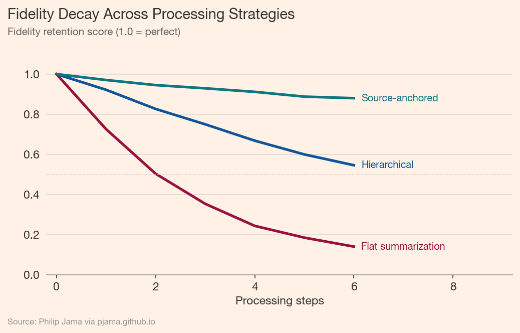
The following visualization compares three processing strategies across multiple steps. Flat summarization -- where each step compresses the previous output -- shows steep fidelity decay. Hierarchical approaches, which maintain multiple levels of detail, degrade more slowly. Source-anchored strategies, which re-consult the original at each step, remain nearly flat.

Show Python source

import math
import matplotlib
matplotlib.use('Agg')
import matplotlib.pyplot as plt
import random

random.seed(42)

FT_BG = '#FFF1E5'
plt.rcParams.update({
    'figure.facecolor': FT_BG,
    'axes.facecolor': FT_BG,
    'savefig.facecolor': FT_BG,
    'font.family': 'sans-serif',
    'font.sans-serif': ['Helvetica Neue', 'Arial', 'DejaVu Sans'],
    'font.size': 11,
    'axes.spines.top': False,
    'axes.spines.right': False,
    'axes.spines.left': False,
    'axes.spines.bottom': True,
    'axes.linewidth': 0.8,
    'axes.edgecolor': '#999999',
    'axes.labelcolor': '#333333',
    'xtick.color': '#333333',
    'ytick.color': '#333333',
    'text.color': '#333333',
})

steps = list(range(0, 7))

# Flat summarization: steep exponential decay
flat = [1.0]
for i in range(1, 7):
    flat.append(flat[-1] * 0.72 + random.uniform(-0.02, 0.02))

# Hierarchical: moderate decay
hier = [1.0]
for i in range(1, 7):
    hier.append(hier[-1] * 0.91 + random.uniform(-0.015, 0.015))

# Source-anchored: near-flat
anchored = [1.0]
for i in range(1, 7):
    anchored.append(max(0.88, anchored[-1] * 0.98 + random.uniform(-0.01, 0.01)))

fig, ax = plt.subplots(figsize=(8, 4.5))

ax.plot(steps, flat, color='#990F3D', linewidth=2.5)
ax.plot(steps, hier, color='#0F5499', linewidth=2.5)
ax.plot(steps, anchored, color='#0D7680', linewidth=2.5)

# Direct labels at right edge
ax.text(6.15, flat[-1], 'Flat summarization', color='#990F3D', fontsize=9.5, va='center', fontweight='bold')
ax.text(6.15, hier[-1], 'Hierarchical', color='#0F5499', fontsize=9.5, va='center', fontweight='bold')
ax.text(6.15, anchored[-1], 'Source-anchored', color='#0D7680', fontsize=9.5, va='center', fontweight='bold')

ax.set_xlim(-0.2, 9.2)
ax.set_ylim(0, 1.08)
ax.set_xlabel('Processing steps')
ax.set_ylabel('')
ax.yaxis.grid(True, color='#CCCCCC', linewidth=0.8, alpha=0.6)
ax.set_axisbelow(True)
ax.tick_params(left=False)
ax.axhline(y=0.5, color='#CCCCCC', linestyle='--', linewidth=0.8, alpha=0.6)

# FT-style headline title
fig.text(0.06, 0.97, 'Fidelity Decay Across Processing Strategies', fontsize=14, fontweight='bold', va='top')
fig.text(0.06, 0.91, 'Fidelity retention score (1.0 = perfect)', fontsize=10, color='#666666', va='top')

fig.subplots_adjust(top=0.82, bottom=0.18)
fig.text(0.06, 0.03, 'Source: Philip Jama via pjama.github.io', fontsize=8, color='#999999', va='bottom')
fig.savefig('fidelity_decay.png', dpi=150, facecolor=FT_BG, bbox_inches='tight')

print('wrote fidelity_decay.png')

Signal and Noise in Context

Token Budget as Bandwidth

A context window is a communication channel with finite bandwidth. Every token spent on irrelevant context is noise that dilutes the signal. Packing 128k tokens with marginally relevant documents does not give the model more information -- it gives it more noise to filter, lowering the signal-to-noise ratio of the entire prompt.

The analogy to Shannon's channel capacity is direct. A channel has a maximum rate at which information can be reliably transmitted. Exceeding that rate does not increase throughput; it increases errors. Similarly, stuffing a context window past the point of useful information does not improve output quality -- it degrades it. The model's attention becomes a scarce resource spread across too many tokens.

The Relevance-Completeness Tension

Prompt construction faces the classic precision-recall tradeoff. High precision (only the most relevant chunks) risks missing context the model needs. High recall (include everything plausibly related) floods the window with noise. Neither extreme produces high-fidelity output.

The resolution is tiered context: full source text for high-relevance documents, structured summaries for supporting material, and exclusion of the rest. This mirrors how human analysts work -- reading primary sources in full while consulting summaries of background material. The tiers are an explicit bandwidth allocation: spend tokens where they carry the most signal.

Strategies for Preserving Fidelity

Structured Source Attribution

Facts that carry inline provenance survive summarization better than naked claims. "Revenue grew 12.3% (Source: Q3 Report, Table 2)" is harder for a summarizer to reduce to "revenue grew significantly" because the attribution signals precision. Embedding provenance directly in content -- rather than in footnotes or metadata -- keeps it in the signal path where the model processes it.

This is a form of redundant encoding. The source tag carries no new information about revenue, but it encodes a constraint: this number has a specific origin and should be preserved exactly. Structured attribution raises the cost of lossy compression by making the loss visible.

Hierarchical Summarization

A single flat summary discards detail uniformly. Hierarchical summarization maintains multiple levels: a one-paragraph executive summary, a section-level summary with key figures, and the full source. Different tasks draw from different levels. A routing question needs only the top level; a fact-checking task needs the full source.

This maps directly to the multi-level retrieval strategy in GraphRAG, where community summaries at different granularities serve different query types. The principle is the same: preserve multiple resolutions of the signal rather than committing to a single lossy compression.

Chain-of-Thought as Signal

Chain-of-thought prompting is often framed as a reasoning improvement. It also serves as a fidelity strategy. When a model shows its intermediate steps, each step is inspectable -- we can verify that the source signal survived the transformation. Hidden reasoning hides errors. If a model jumps from source document to conclusion without visible intermediate steps, there is no way to detect where fidelity loss occurred.

The tradeoff is token cost. Showing work consumes context window bandwidth. But the tokens spent on chain-of-thought are signal -- they make the processing chain transparent and auditable. This is a bandwidth allocation decision, not waste.

Retrieval over Compression

Retrieval-augmented generation restores fidelity by re-consulting the source rather than relying on degraded copies. Each retrieval step refreshes the context with original-fidelity content, resetting the drift that accumulates through summarization chains. This is why RAG pipelines often outperform systems that pre-summarize their knowledge base: they trade compute for fidelity.

The knowledge graph approaches in Knowledge Graphs from Text and GraphRAG extend this principle. Structured extraction preserves entity relationships and provenance that flat text retrieval might miss. The graph is a fidelity-preserving representation -- it captures the relational structure of the source, not just its surface text.

Explicit Preservation Contracts

When specific facts must survive a processing step verbatim, name them explicitly in the prompt. "The following numbers must appear unchanged in your output: 12.3% revenue growth, $4.2M ARR, 847 enterprise accounts." This is invariant specification for LLM pipelines -- the same discipline as writing assertions in software, applied to information processing.

Preservation contracts work because they convert implicit expectations into explicit constraints. Without them, the model optimizes for fluency and coherence, which may conflict with numerical precision. With them, the model has a clear signal about what the consumer of its output needs preserved.

Measuring Fidelity Loss

Factual Consistency Checking

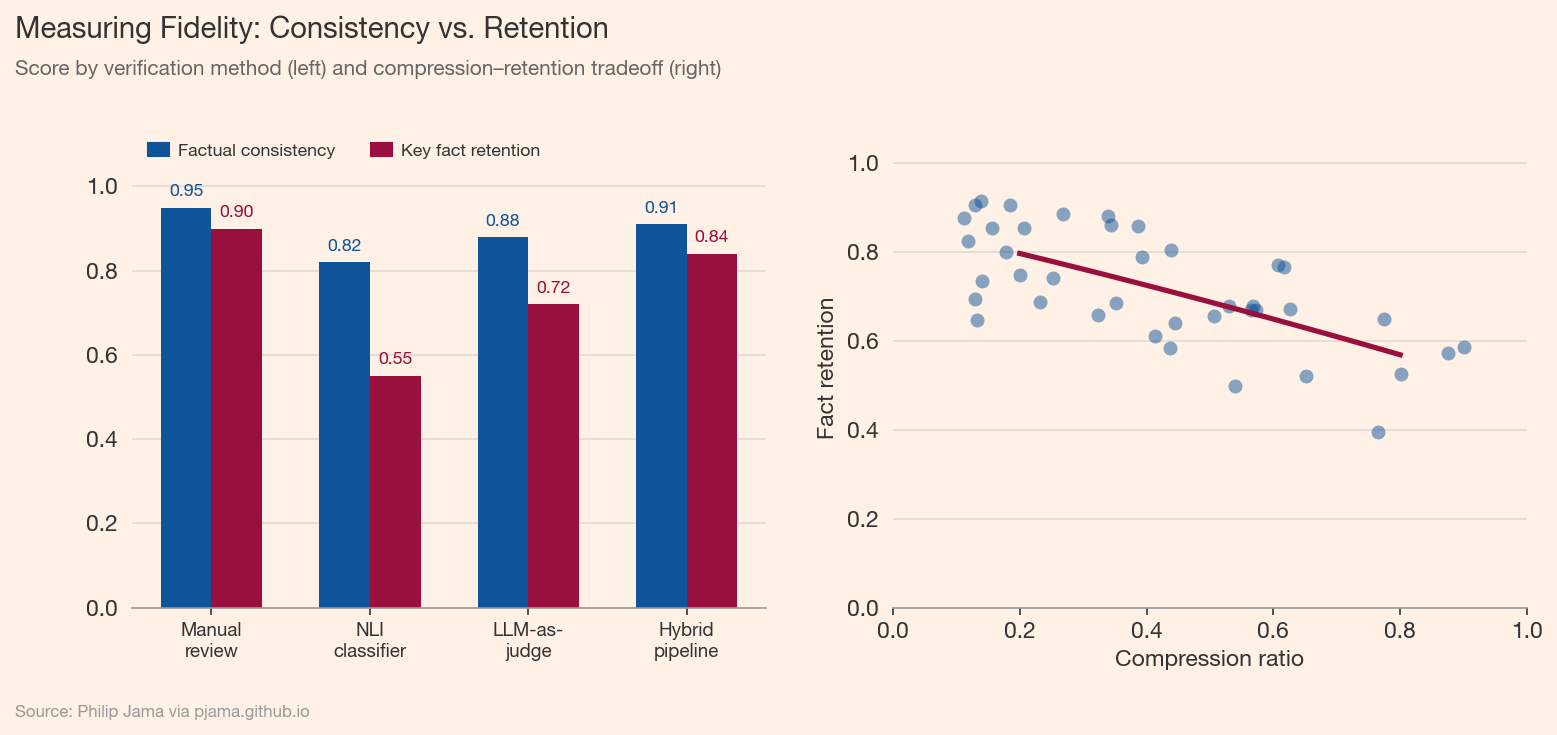
Fidelity measurement compares output against source. Three approaches, in order of increasing automation: manual review against source documents, natural language inference (NLI) models that classify output sentences as entailed, contradicted, or neutral relative to the source, and LLM-as-judge evaluation where a separate model checks faithfulness. Each trades cost for coverage.

The NLI approach is attractive for pipeline monitoring: run every output through an entailment classifier and flag contradictions automatically. But entailment checks only catch one class of fidelity failure -- they detect when the output says something the source does not support. They do not detect when the output omits something the source says.

The Asymmetry of Loss: Detecting Omissions

Detecting additions (hallucination) is easier than detecting omissions. A contradicted claim triggers NLI classifiers and fact-checkers. A missing fact triggers nothing. Yet a technically accurate summary that omits the key finding is a fidelity failure no contradiction check catches.

This asymmetry means that fidelity measurement must include recall-oriented checks: does the output contain the critical facts from the source? This requires defining what "critical" means up front -- another argument for explicit preservation contracts. Without a specification of what must survive, there is no way to measure whether it did.

The following visualization compares factual consistency (contradiction detection) against key fact retention (recall) across processing methods, and shows the relationship between compression ratio and fact retention.

Show Python source

import matplotlib
matplotlib.use('Agg')
import matplotlib.pyplot as plt
import matplotlib.patches as mpatches
import random

random.seed(7)

FT_BG = '#FFF1E5'
plt.rcParams.update({
    'figure.facecolor': FT_BG,
    'axes.facecolor': FT_BG,
    'savefig.facecolor': FT_BG,
    'font.family': 'sans-serif',
    'font.sans-serif': ['Helvetica Neue', 'Arial', 'DejaVu Sans'],
    'font.size': 11,
    'axes.spines.top': False,
    'axes.spines.right': False,
    'axes.spines.left': False,
    'axes.spines.bottom': True,
    'axes.linewidth': 0.8,
    'axes.edgecolor': '#999999',
    'axes.labelcolor': '#333333',
    'xtick.color': '#333333',
    'ytick.color': '#333333',
    'text.color': '#333333',
})

methods = ['Manual\nreview', 'NLI\nclassifier', 'LLM-as-\njudge', 'Hybrid\npipeline']
consistency = [0.95, 0.82, 0.88, 0.91]
retention = [0.90, 0.55, 0.72, 0.84]

# Scatter data: compression ratio vs fact retention
n = 40
comp_ratios = [random.uniform(0.08, 0.92) for _ in range(n)]
fact_ret = []
for cr in comp_ratios:
    base = 0.95 - 0.6 * cr + 0.15 * cr * cr
    noise = random.gauss(0, 0.09)
    fact_ret.append(max(0.15, min(1.0, base + noise)))

fig, (ax1, ax2) = plt.subplots(1, 2, figsize=(12, 5))

# Bar chart
x_pos = list(range(len(methods)))
w = 0.32
bars1 = ax1.bar([p - w/2 for p in x_pos], consistency, w, color='#0F5499', linewidth=0)
bars2 = ax1.bar([p + w/2 for p in x_pos], retention, w, color='#990F3D', linewidth=0)

# Value labels above bars
for bar in bars1:
    ax1.text(bar.get_x() + bar.get_width()/2, bar.get_height() + 0.02,
             f'{bar.get_height():.2f}', ha='center', va='bottom', fontsize=8.5, color='#0F5499', fontweight='bold')
for bar in bars2:
    ax1.text(bar.get_x() + bar.get_width()/2, bar.get_height() + 0.02,
             f'{bar.get_height():.2f}', ha='center', va='bottom', fontsize=8.5, color='#990F3D', fontweight='bold')

ax1.set_xticks(x_pos)
ax1.set_xticklabels(methods, fontsize=9)
ax1.set_ylim(0, 1.14)
ax1.set_ylabel('')
ax1.yaxis.grid(True, color='#CCCCCC', linewidth=0.8, alpha=0.6)
ax1.set_axisbelow(True)
ax1.tick_params(left=False)

# Horizontal legend with colored squares
p1 = mpatches.Patch(color='#0F5499', label='Factual consistency')
p2 = mpatches.Patch(color='#990F3D', label='Key fact retention')
ax1.legend(handles=[p1, p2], loc='upper left', fontsize=8.5, frameon=False, ncol=2, handlelength=1.2, handletextpad=0.5)

# Scatter plot
import numpy as np
ax2.scatter(comp_ratios, fact_ret, color='#0F5499', alpha=0.5, s=45, linewidths=0)
# Polynomial trend line across full range
coeffs = np.polyfit(comp_ratios, fact_ret, 2)
xfit = np.linspace(0.2, 0.8, 100)
yfit = np.polyval(coeffs, xfit)
ax2.plot(xfit, yfit, color='#990F3D', linewidth=2.5)
ax2.set_xlim(0, 1)
ax2.set_ylim(0, 1.08)
ax2.set_xlabel('Compression ratio')
ax2.set_ylabel('Fact retention')
ax2.yaxis.grid(True, color='#CCCCCC', linewidth=0.8, alpha=0.6)
ax2.set_axisbelow(True)
ax2.tick_params(left=False)

# FT-style headline titles
fig.text(0.06, 0.97, 'Measuring Fidelity: Consistency vs. Retention', fontsize=14, fontweight='bold', va='top')
fig.text(0.06, 0.91, 'Score by verification method (left) and compression\u2013retention tradeoff (right)', fontsize=10, color='#666666', va='top')

fig.subplots_adjust(top=0.82, bottom=0.18, wspace=0.2)
fig.text(0.06, 0.03, 'Source: Philip Jama via pjama.github.io', fontsize=8, color='#999999', va='bottom')
fig.savefig('fidelity_measurement.png', dpi=150, facecolor=FT_BG, bbox_inches='tight')

print('wrote fidelity_measurement.png')

Architectural Patterns

Source-of-Truth Layers

High-fidelity systems maintain a source-of-truth layer: canonical data that is never summarized away. Summaries are caches, not replacements. When a downstream process needs precision, it queries the source layer directly. When it needs speed or breadth, it reads from the summary cache.

The parallel to database normalization is direct. A normalized schema stores each fact once and derives views as needed. Denormalized caches trade fidelity for performance. The same tradeoff applies to LLM pipelines: pre-computed summaries are denormalized caches of the source documents. Treat them accordingly -- use them for routing and overview, not for precision tasks.

Tiered Context Architecture

A practical implementation uses three tiers. Tier 1: full source text for the most relevant documents. Tier 2: structured summaries (with key figures and source attribution) for supporting context. Tier 3: metadata and routing information (titles, dates, relevance scores) for everything else. The tier is selected by task type and relevance score.

This maps to the local vs. global retrieval distinction in GraphRAG. Local queries need Tier 1 (specific passages from specific documents). Global queries need Tier 2 (community summaries that span the corpus). Routing queries need only Tier 3. Matching the tier to the task prevents both fidelity loss (from over-compression) and noise (from under-filtering).

Provenance and Versioning

Every derived artifact should record its derivation chain: which source documents contributed, what prompt produced it, which model version ran, and when. This is version control for information processing. When a source document updates, we can identify which downstream artifacts are stale and re-derive them.

The knowledge graph approach in LLM Knowledge Graphs provides a natural structure for provenance tracking. Entities and relationships extracted from source documents carry their source attribution as graph metadata. When the source changes, the affected subgraph is identifiable and can be selectively refreshed.

When to Re-derive vs. Cache

Cache invalidation is a fidelity management decision. Re-derive when the source document has changed, when the task requires numerical precision, or when the cached artifact is multiple hops from the original. Cache when the source is stable, the task tolerates approximation, and the derivation is expensive.

A useful heuristic: count the hops between the cached artifact and its source. One hop (direct summary) is usually safe to cache. Two hops (summary of summaries) warrants periodic re-derivation. Three or more hops should trigger re-derivation from source for any precision-sensitive task. The hop count is a proxy for accumulated drift.

Larger context windows shift the engineering problem from "what fits" to "what matters." A 200k-token window does not eliminate fidelity concerns -- it changes them. The noise floor rises with context length, attention diffuses over more tokens, and the temptation to include everything replaces the discipline of selecting what is relevant. The signal engineering mindset -- measure what you need, preserve it deliberately, verify it survived -- remains the core discipline regardless of how many tokens the model can hold.