Philip Jama

Articles /Network Graph Analysis /Part 2

Community Detection in Social Graphs

Modularity, Louvain, and stochastic block models for finding structure

Graph TheoryPythonCommunity DetectionNetwork Analysis

Most real networks are not uniform: they contain densely connected subgroups with sparser links between them. Identifying these communities reveals functional modules in biological networks, social circles in friendship graphs, and topic clusters in citation networks. This article covers the algorithmic and generative approaches to community detection, drawing on techniques used in the Calendar Graph project ↗.

What Is Community Structure

A community (or cluster, or module) is a group of nodes more densely connected internally than externally. The intuition is simple, but formalizing it requires a quality function: a way to score a proposed partition. The most widely used is modularity.

Modularity and the Louvain Algorithm

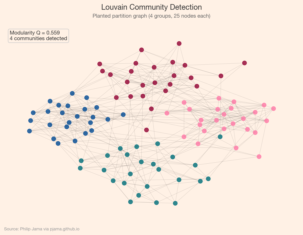
Modularity Q compares the fraction of edges within communities to the expected fraction under a random null model. Values near 0 mean no better than random; values approaching 1 indicate strong community structure. The Louvain algorithm greedily optimizes modularity in two phases: local node moves followed by community aggregation, iterating until convergence. It scales well to large networks and remains a go-to baseline.

Planted partition graph with Louvain-detected communities colored
Show Python source
import networkx as nx
import numpy as np
import matplotlib
matplotlib.use('Agg')
import matplotlib.pyplot as plt
import random

FT_BG = '#FFF1E5'
FT_CLARET = '#990F3D'
FT_OXFORD = '#0F5499'
FT_TEAL = '#0D7680'
FT_CANDY = '#FF7FAA'

plt.rcParams.update({
    'figure.facecolor': FT_BG,
    'axes.facecolor': FT_BG,
    'savefig.facecolor': FT_BG,
    'font.family': 'sans-serif',
    'font.sans-serif': ['Helvetica Neue', 'Arial', 'sans-serif'],
    'axes.spines.top': False,
    'axes.spines.right': False,
})

random.seed(42)
np.random.seed(42)

G = nx.planted_partition_graph(4, 25, 0.3, 0.02, seed=42)
communities = nx.community.louvain_communities(G, seed=42)
modularity = nx.community.modularity(G, communities)

ft_palette = [FT_OXFORD, FT_CLARET, FT_TEAL, FT_CANDY]
node_colors = ['#999999'] * len(G)
for i, comm in enumerate(communities):
    for n in comm:
        node_colors[n] = ft_palette[i % len(ft_palette)]

fig, ax = plt.subplots(figsize=(8, 6))
pos = nx.spring_layout(G, seed=42)
nx.draw_networkx_edges(G, pos, ax=ax, alpha=0.15, width=0.5)
nx.draw_networkx_nodes(G, pos, ax=ax, node_color=node_colors,
                       node_size=60, alpha=0.85)
ax.text(0.02, 0.98, f'Modularity Q = {modularity:.3f}\n{len(communities)} communities detected',
        transform=ax.transAxes, va='top', fontsize=10, color='#333333',
        bbox=dict(boxstyle='round', facecolor=FT_BG, edgecolor='#cccccc', alpha=0.9))
ax.set_axis_off()

fig.text(0.5, 0.97, 'Louvain Community Detection',
         ha='center', fontsize=14, fontweight='bold', color='#333333')
fig.text(0.5, 0.935, 'Planted partition graph (4 groups, 25 nodes each)',
         ha='center', fontsize=10, color='#666666')
fig.text(0.02, 0.01, 'Source: Philip Jama via pjama.github.io',
         fontsize=8, color='#999999', ha='left')
fig.tight_layout(rect=[0, 0.03, 1, 0.92])
fig.savefig('louvain_communities.png', dpi=150, bbox_inches='tight')

print('wrote louvain_communities.png')

Stochastic Block Models

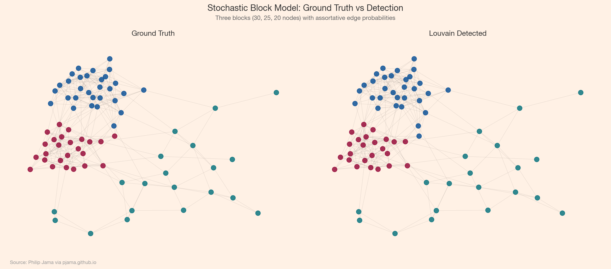
Where Louvain optimizes a heuristic score, Stochastic Block Models (SBMs) take a generative approach: they posit that each node belongs to a latent block, and edges form with probabilities that depend on block membership. Fitting an SBM means inferring which block assignment best explains the observed edges. SBMs can detect disassortative structure (groups that connect between more than within) that modularity-based methods miss.

Hierarchical Community Detection

Communities often nest: a university has departments, which have research groups, which have labs. Hierarchical methods: dendrogram-based agglomerative clustering or nested SBMs capture this multi-scale structure. The Calendar Graph project ↗ uses hierarchical clustering to reveal organizational layers in interaction networks.

Stochastic block model: inferred vs. ground-truth communities
Show Python source
import networkx as nx
import numpy as np
import matplotlib
matplotlib.use('Agg')
import matplotlib.pyplot as plt
import random

FT_BG = '#FFF1E5'
FT_CLARET = '#990F3D'
FT_OXFORD = '#0F5499'
FT_TEAL = '#0D7680'

plt.rcParams.update({
    'figure.facecolor': FT_BG,
    'axes.facecolor': FT_BG,
    'savefig.facecolor': FT_BG,
    'font.family': 'sans-serif',
    'font.sans-serif': ['Helvetica Neue', 'Arial', 'sans-serif'],
    'axes.spines.top': False,
    'axes.spines.right': False,
})

random.seed(42)
np.random.seed(42)

sizes = [30, 25, 20]
probs = [[0.3, 0.02, 0.01], [0.02, 0.35, 0.02], [0.01, 0.02, 0.25]]
G = nx.stochastic_block_model(sizes, probs, seed=42)

ft_palette = [FT_OXFORD, FT_CLARET, FT_TEAL]
gt_colors = [ft_palette[0]]*30 + [ft_palette[1]]*25 + [ft_palette[2]]*20

detected = nx.community.louvain_communities(G, seed=42)
det_colors = ['#999999'] * len(G)
for i, comm in enumerate(detected):
    for n in comm:
        det_colors[n] = ft_palette[i % len(ft_palette)]

pos = nx.spring_layout(G, seed=42)
fig, (ax1, ax2) = plt.subplots(1, 2, figsize=(14, 6))

nx.draw_networkx_edges(G, pos, ax=ax1, alpha=0.1, width=0.5)
nx.draw_networkx_nodes(G, pos, ax=ax1, node_color=gt_colors,
                       node_size=60, alpha=0.85)
ax1.set_title('Ground Truth', fontsize=12, fontweight='600', color='#333333', pad=8)
ax1.set_axis_off()

nx.draw_networkx_edges(G, pos, ax=ax2, alpha=0.1, width=0.5)
nx.draw_networkx_nodes(G, pos, ax=ax2, node_color=det_colors,
                       node_size=60, alpha=0.85)
ax2.set_title('Louvain Detected', fontsize=12, fontweight='600', color='#333333', pad=8)
ax2.set_axis_off()

fig.text(0.5, 0.97, 'Stochastic Block Model: Ground Truth vs Detection',
         ha='center', fontsize=14, fontweight='bold', color='#333333')
fig.text(0.5, 0.935, 'Three blocks (30, 25, 20 nodes) with assortative edge probabilities',
         ha='center', fontsize=10, color='#666666')
fig.text(0.02, 0.01, 'Source: Philip Jama via pjama.github.io',
         fontsize=8, color='#999999', ha='left')
fig.tight_layout(rect=[0, 0.03, 1, 0.92])
fig.savefig('sbm_communities.png', dpi=150, bbox_inches='tight')

print('wrote sbm_communities.png')

Application to Organizational Networks

Community detection maps directly onto organizational analysis. In a collaboration or communication graph, detected communities might reveal cross-functional teams, information silos, or informal influence groups. Comparing the algorithmic partition to the formal org chart often surfaces surprising structure: bridging individuals, isolated clusters, or shadow hierarchies. The Calendar Graph project ↗ applies these techniques to real organizational communication data.

Collaborate

If you're exploring related work and need hands-on help, I'm open to consulting and advisory. Get in touch