Philip Jama

Articles /Network Graph Analysis /Part 3

Centrality, Influence, and Spectral Methods

Who matters in a network: from degree counts to the graph Laplacian

Graph TheoryPythonCentralitySpectral AnalysisNetwork Analysis

Not all nodes are equal. Some sit at the crossroads of information flow; others anchor tightly-knit clusters. Centrality measures quantify importance from different angles, while spectral methods reveal global structure through the eigenvalues and eigenvectors of graph matrices. This article covers both, connecting to resistance distance and betweenness concepts from the Calendar Graph project ↗. It builds on the community structure ideas from Part 2 (Community Detection in Social Graphs).

Who Matters in a Network

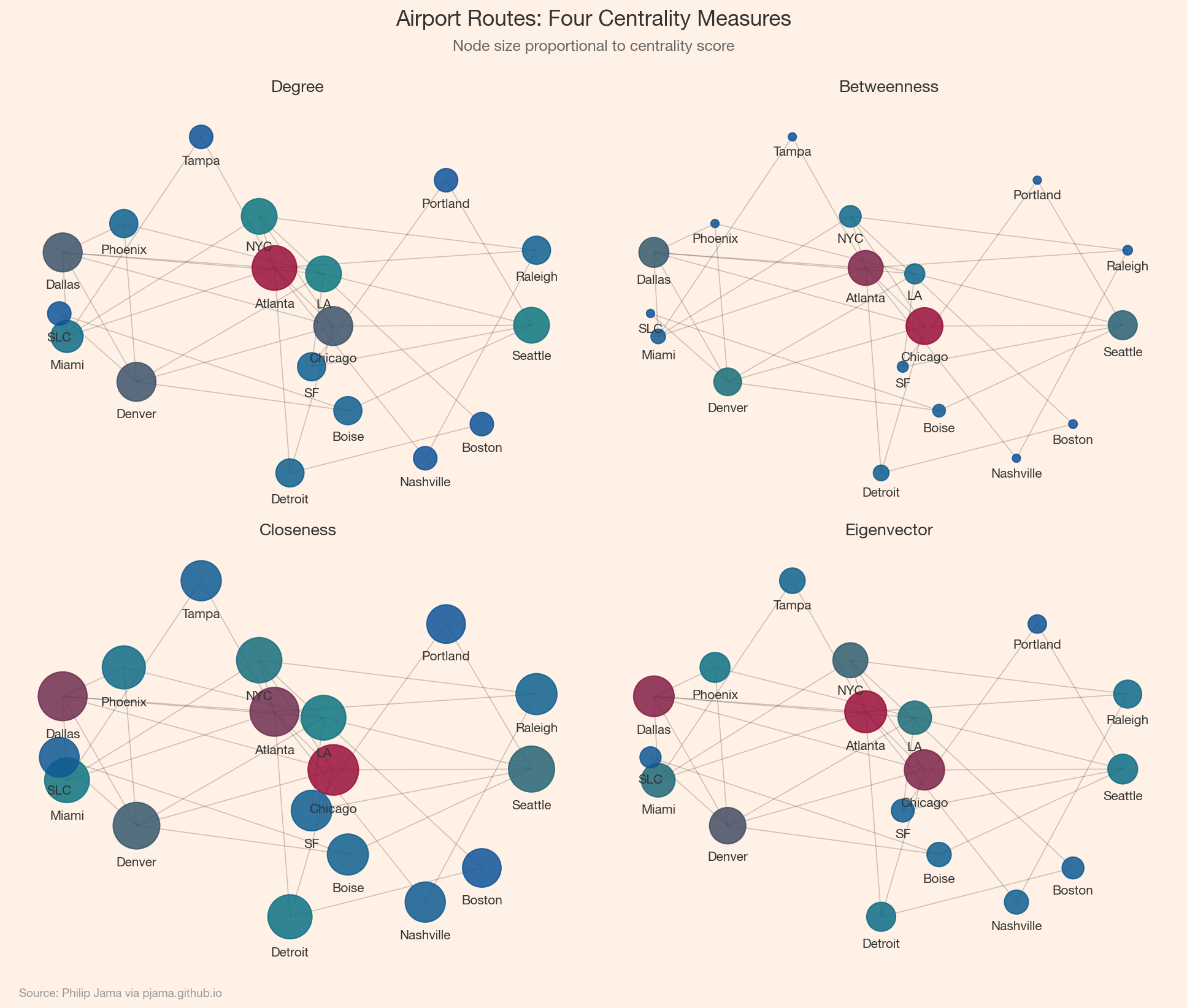
"Important" depends on context. A node might be important because it has many connections (degree), because it lies on many shortest paths (betweenness), because it is close to all others (closeness), or because it connects to other important nodes (eigenvector centrality). Each definition answers a different question about influence and access.

Degree, Betweenness, Closeness, Eigenvector Centrality

  • Degree centrality: simply the number (or fraction) of edges. High-degree nodes are hubs.
  • Betweenness centrality: the fraction of all shortest paths that pass through a node. High betweenness indicates a bridge or broker.
  • Closeness centrality: the inverse of the average shortest-path distance to all other nodes. High closeness means fast access.
  • Eigenvector centrality: a node scores high if its neighbors also score high. This recursive definition is solved as the leading eigenvector of the adjacency matrix.

PageRank

PageRank is a damped variant of eigenvector centrality designed for directed graphs. A random walker follows outgoing links with probability d and teleports to a random node with probability 1−d. The stationary distribution of this walk defines PageRank. It famously powered early Google search and remains useful for ranking nodes in any directed network.

Airport route network with nodes sized by degree, betweenness, closeness, and eigenvector centrality
Show Python source
import networkx as nx
import numpy as np
import matplotlib
matplotlib.use('Agg')
import matplotlib.pyplot as plt
from matplotlib.colors import LinearSegmentedColormap

FT_BG = '#FFF1E5'
FT_CLARET = '#990F3D'
FT_OXFORD = '#0F5499'
FT_TEAL = '#0D7680'

plt.rcParams.update({
    'figure.facecolor': FT_BG,
    'axes.facecolor': FT_BG,
    'savefig.facecolor': FT_BG,
    'font.family': 'sans-serif',
    'font.sans-serif': ['Helvetica Neue', 'Arial', 'sans-serif'],
    'axes.spines.top': False,
    'axes.spines.right': False,
})

# Synthetic airport route network
cities = ['Atlanta', 'Chicago', 'Denver', 'Dallas', 'LA', 'NYC',
          'Seattle', 'Miami', 'Phoenix', 'Detroit', 'Boston', 'SF',
          'Portland', 'SLC', 'Nashville', 'Boise', 'Tampa', 'Raleigh']
routes = [
    ('Atlanta', 'Chicago'), ('Atlanta', 'Dallas'), ('Atlanta', 'NYC'),
    ('Atlanta', 'Miami'), ('Atlanta', 'Nashville'), ('Atlanta', 'Tampa'),
    ('Atlanta', 'Raleigh'), ('Atlanta', 'Detroit'),
    ('Chicago', 'Denver'), ('Chicago', 'NYC'), ('Chicago', 'Detroit'),
    ('Chicago', 'Dallas'), ('Chicago', 'Seattle'),
    ('Denver', 'Dallas'), ('Denver', 'LA'), ('Denver', 'SLC'),
    ('Denver', 'Phoenix'), ('Denver', 'Boise'),
    ('Dallas', 'LA'), ('Dallas', 'Miami'), ('Dallas', 'Phoenix'),
    ('LA', 'SF'), ('LA', 'Seattle'), ('LA', 'Phoenix'),
    ('NYC', 'Boston'), ('NYC', 'Miami'), ('NYC', 'Raleigh'),
    ('Seattle', 'Portland'), ('Seattle', 'SF'), ('Seattle', 'Boise'),
    ('SF', 'Portland'), ('SLC', 'Boise'), ('Nashville', 'Raleigh'),
    ('Miami', 'Tampa'), ('Detroit', 'Boston')
]

G = nx.Graph()
G.add_nodes_from(cities)
G.add_edges_from(routes)
pos = nx.spring_layout(G, seed=42, k=1.8)

deg = nx.degree_centrality(G)
bet = nx.betweenness_centrality(G)
clo = nx.closeness_centrality(G)
eig = nx.eigenvector_centrality(G, max_iter=1000)

# FT-inspired colormap: Oxford blue to Teal to Claret
ft_cmap = LinearSegmentedColormap.from_list('ft', [FT_OXFORD, FT_TEAL, FT_CLARET])

measures = [('Degree', deg), ('Betweenness', bet),
            ('Closeness', clo), ('Eigenvector', eig)]

fig, axes = plt.subplots(2, 2, figsize=(13, 11))
for ax, (name, cent) in zip(axes.flat, measures):
    vals = [cent[nd] for nd in G.nodes()]
    sizes = [v * 2500 + 40 for v in vals]
    nx.draw_networkx_edges(G, pos, ax=ax, alpha=0.2, width=0.8)
    nx.draw_networkx_nodes(G, pos, ax=ax, node_size=sizes,
                           node_color=vals, cmap=ft_cmap, alpha=0.85)
    # Offset labels below nodes: radius in points = sqrt(size / pi)
    import math
    node_list = list(G.nodes())
    for j, nd in enumerate(node_list):
        x, y = pos[nd]
        r_pts = math.sqrt(sizes[j] / math.pi)  # radius in points
        ax.annotate(nd, (x, y), xytext=(0, -(r_pts + 4)),
                    textcoords='offset points', ha='center', va='top',
                    fontsize=10, color='#333333')
    ax.set_title(name, fontsize=13, fontweight='600', color='#333333', pad=8)
    ax.set_axis_off()

fig.text(0.5, 0.97, 'Airport Routes: Four Centrality Measures',
         ha='center', fontsize=17, fontweight='bold', color='#333333')
fig.text(0.5, 0.945, 'Node size proportional to centrality score',
         ha='center', fontsize=12, color='#666666')
fig.text(0.02, 0.01, 'Source: Philip Jama via pjama.github.io',
         fontsize=9, color='#999999', ha='left')
fig.tight_layout(rect=[0, 0.03, 1, 0.93])
fig.savefig('centrality_comparison.png', dpi=150, bbox_inches='tight')

print('wrote centrality_comparison.png')

Resistance Distance and Electrical Network Theory

Imagine the graph as a resistor network where each edge is a 1-ohm resistor. The resistance distance between two nodes is the effective resistance between them. Unlike shortest-path distance, resistance distance accounts for all paths and their redundancy: more parallel paths mean lower resistance. This makes it a robust measure of connectivity that is less sensitive to single-edge failures. The Calendar Graph project ↗ uses resistance distance to identify structurally important connections in organizational networks.

Spectral Analysis: Graph Laplacian and Fiedler Vector

The graph Laplacian L = D − A (degree matrix minus adjacency matrix) encodes global structure in its eigenvalues. The smallest eigenvalue is always 0 (with eigenvector proportional to the all-ones vector). The second-smallest eigenvalue, the algebraic connectivity, measures how well-connected the graph is. Its corresponding eigenvector, the Fiedler vector, provides a one-dimensional embedding that naturally partitions the graph into two clusters. This spectral bisection is the foundation of spectral clustering.

Graph colored by Fiedler vector sign showing spectral bisection
Show Python source
import networkx as nx
import numpy as np
import matplotlib
matplotlib.use('Agg')
import matplotlib.pyplot as plt
import random

FT_BG = '#FFF1E5'
FT_CLARET = '#990F3D'
FT_OXFORD = '#0F5499'
FT_TEAL = '#0D7680'

plt.rcParams.update({
    'figure.facecolor': FT_BG,
    'axes.facecolor': FT_BG,
    'savefig.facecolor': FT_BG,
    'font.family': 'sans-serif',
    'font.sans-serif': ['Helvetica Neue', 'Arial', 'sans-serif'],
    'axes.spines.top': False,
    'axes.spines.right': False,
})

random.seed(42)
np.random.seed(42)

G = nx.planted_partition_graph(2, 30, 0.35, 0.05, seed=42)
L = nx.laplacian_matrix(G).toarray().astype(float)
eigenvalues, eigenvectors = np.linalg.eigh(L)
fiedler = eigenvectors[:, 1]
sorted_idx = np.argsort(fiedler)
colors = [FT_OXFORD if f >= 0 else FT_CLARET for f in fiedler]

fig, (ax1, ax2) = plt.subplots(1, 2, figsize=(14, 5))

# Fiedler vector bar chart
bar_colors = [FT_OXFORD if f >= 0 else FT_CLARET for f in fiedler[sorted_idx]]
ax1.bar(range(len(fiedler)), fiedler[sorted_idx], color=bar_colors, alpha=0.85)
ax1.axhline(0, color='#333333', linewidth=0.8, linestyle='--')
ax1.set_xlabel('Node (sorted)', fontsize=12, color='#333333')
ax1.set_ylabel('Fiedler value', fontsize=12, color='#333333')
ax1.spines['left'].set_color('#cccccc')
ax1.spines['bottom'].set_color('#cccccc')
ax1.tick_params(colors='#666666', labelsize=10)
ax1.yaxis.grid(True, alpha=0.2, color='#999999')
ax1.set_axisbelow(True)

# Spectral bisection graph
pos = nx.spring_layout(G, seed=42)
nx.draw_networkx_edges(G, pos, ax=ax2, alpha=0.15, width=0.5)
nx.draw_networkx_nodes(G, pos, ax=ax2, node_color=colors,
                       node_size=80, alpha=0.85)
ax2.text(0.02, 0.98, f'Algebraic connectivity: {eigenvalues[1]:.3f}',
         transform=ax2.transAxes, va='top', fontsize=11, color='#333333',
         bbox=dict(boxstyle='round', facecolor=FT_BG, edgecolor='#cccccc', alpha=0.9))
ax2.set_axis_off()

fig.text(0.5, 0.98, 'Spectral Bisection via the Fiedler Vector',
         ha='center', fontsize=17, fontweight='bold', color='#333333')
fig.text(0.5, 0.935, 'Planted partition graph (2 communities, 30 nodes each)',
         ha='center', fontsize=12, color='#666666')
fig.text(0.02, 0.01, 'Source: Philip Jama via pjama.github.io',
         fontsize=9, color='#999999', ha='left')
fig.tight_layout(rect=[0, 0.04, 1, 0.92])
fig.savefig('spectral_fiedler.png', dpi=150, bbox_inches='tight')

print('wrote spectral_fiedler.png')

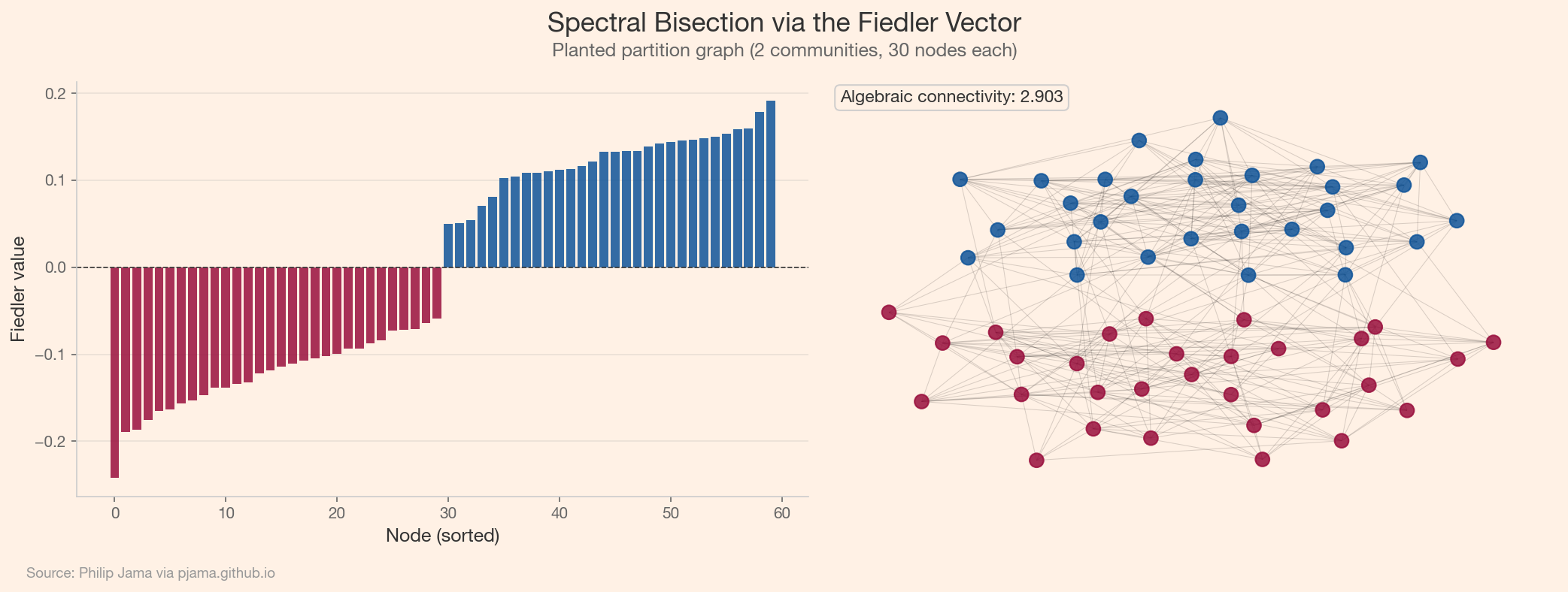
This technique has direct practical value. Chip designers use spectral bisection to partition circuits onto separate dies, minimizing the number of wires that cross the cut. Network engineers apply it to split backbone topologies into failure-independent zones. In social network analysis, the Fiedler vector reveals the most natural ideological or organizational fault line in a community — the split that would require severing the fewest relationships. The sign of each node's Fiedler value assigns it to one side; the magnitude indicates how strongly it belongs there. Nodes near zero sit on the boundary and are often the most interesting: they bridge the two groups.

Centrality and spectral methods characterize structure in existing graphs. What if the graph doesn't exist yet and has to be built from raw text?

View all articles in Network Graph Analysis

Collaborate

If you're exploring related work and need hands-on help, I'm open to consulting and advisory. Get in touch