A/B testing allocates traffic equally between variants and waits for a fixed horizon. This is simple, but it has a cost: every user assigned to the worse variant is a missed opportunity. Multi-armed bandits reframe the problem. Instead of testing first and deploying later, bandits learn and earn simultaneously by shifting traffic toward the better-performing arm as evidence accumulates.
The name comes from a row of slot machines ("one-armed bandits") in a casino. Each machine pays out at an unknown rate. The gambler must decide which machines to play and how often, balancing exploration (trying new machines to learn their rates) against exploitation (playing the machine that looks best so far). This explore-exploit tension appears everywhere: ad placement, recommendation systems, clinical trials, and feature rollouts.
The Explore-Exploit Tradeoff
Pure exploration (uniform random allocation) learns quickly but wastes traffic on bad arms. Pure exploitation (always pick the current leader) converges fast but risks locking onto a suboptimal arm before gathering enough evidence. Every bandit algorithm navigates this tradeoff differently.
The key insight: the optimal balance depends on how much uncertainty remains. Early in the experiment, when posteriors are wide, exploration is cheap because you are almost as likely to gain information from any arm. Late in the experiment, when one arm clearly dominates, continued exploration wastes resources.
Thompson Sampling
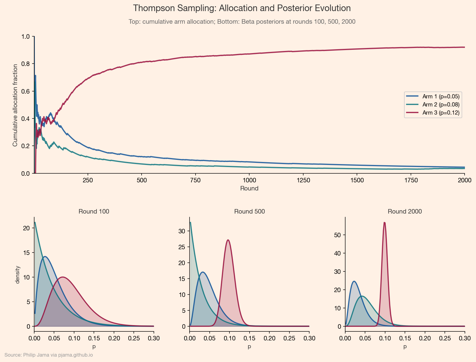
Thompson sampling is a Bayesian bandit algorithm with a remarkably simple rule: on each round, sample a value from each arm's posterior distribution, then play the arm whose sample is highest. Arms with high uncertainty get explored because their samples occasionally land above the current leader. Arms with low expected reward get abandoned because their samples rarely win.
For binary outcomes (click/no-click, convert/not), each arm's posterior is a Beta distribution, exactly as in Part 1 (Online Experiments with a Bayesian Lens). Start with Beta(1, 1) priors, observe successes and failures, and update. Thompson sampling turns those posteriors directly into an allocation policy.
The algorithm in pseudocode:
For each arm k, maintain posterior Beta(a_k, b_k).
At each round, draw theta_k ~ Beta(a_k, b_k) for every arm.
Play the arm with the largest theta_k.
Observe the outcome and update the chosen arm's parameters.
Thompson sampling allocation converging toward the best arm as posteriors narrow Show Python source
import math
import random
import numpy as np
import matplotlib
matplotlib.use('Agg')
import matplotlib.pyplot as plt
import matplotlib.gridspec as gridspec

random.seed(42)
FT_BG = '#FFF1E5'
FT_CLARET = '#990F3D'
FT_OXFORD = '#0F5499'
FT_TEAL = '#0D7680'

plt.rcParams.update({
    'figure.facecolor': FT_BG,
    'axes.facecolor': FT_BG,
    'savefig.facecolor': FT_BG,
    'font.family': 'sans-serif',
    'font.sans-serif': ['Helvetica Neue', 'Arial', 'sans-serif'],
    'axes.spines.top': False,
    'axes.spines.right': False,
})

def beta_pdf(x, a, b):
    x = max(min(x, 1 - 1e-7), 1e-7)
    lg = math.lgamma
    log_pdf = (a - 1) * math.log(x) + (b - 1) * math.log(1 - x) - (
        lg(a) + lg(b) - lg(a + b))
    return math.exp(log_pdf)

true_rates = [0.05, 0.08, 0.12]
arm_names = ['Arm 1 (p=0.05)', 'Arm 2 (p=0.08)', 'Arm 3 (p=0.12)']
arm_colors = [FT_OXFORD, FT_TEAL, FT_CLARET]
K = len(true_rates)
T = 2000

alphas = [1] * K
betas = [1] * K
counts = [0] * K
cumulative_frac = [[] for _ in range(K)]
snapshot_rounds = [100, 500, 2000]
snapshots = {}

for t in range(1, T + 1):
    samples = [random.betavariate(alphas[k], betas[k]) for k in range(K)]
    arm = samples.index(max(samples))
    reward = 1 if random.random() < true_rates[arm] else 0
    alphas[arm] += reward
    betas[arm] += (1 - reward)
    counts[arm] += 1
    for k in range(K):
        cumulative_frac[k].append(counts[k] / t)
    if t in snapshot_rounds:
        snapshots[t] = [(alphas[k], betas[k]) for k in range(K)]

fig = plt.figure(figsize=(11, 8))
gs = gridspec.GridSpec(2, 3, height_ratios=[1.2, 1], hspace=0.35, wspace=0.3)

ax_top = fig.add_subplot(gs[0, :])
rounds = list(range(1, T + 1))
for k in range(K):
    ax_top.plot(rounds, cumulative_frac[k], color=arm_colors[k], linewidth=2,
                label=arm_names[k], alpha=0.85)
ax_top.set_xlim(1, T)
ax_top.set_ylim(0, 1)
ax_top.set_xlabel('Round', fontsize=10, color='#333333')
ax_top.set_ylabel('Cumulative allocation fraction', fontsize=10, color='#333333')
ax_top.legend(fontsize=9, loc='center right', framealpha=0.9)

for i, t_snap in enumerate(snapshot_rounds):
    ax = fig.add_subplot(gs[1, i])
    xs = [j / 500 for j in range(1, 500)]
    for k in range(K):
        a, b = snapshots[t_snap][k]
        ys = [beta_pdf(x, a, b) for x in xs]
        ax.fill_between(xs, ys, color=arm_colors[k], alpha=0.2)
        ax.plot(xs, ys, color=arm_colors[k], linewidth=1.8, alpha=0.85)
    ax.set_xlim(0, 0.3)
    ax.set_xlabel('p', fontsize=9, color='#333333')
    if i == 0:
        ax.set_ylabel('density', fontsize=9, color='#333333')
    ax.set_title(f'Round {t_snap}', fontsize=10, color='#333333')

fig.text(0.5, 0.97, 'Thompson Sampling: Allocation and Posterior Evolution',
         ha='center', fontsize=14, fontweight='bold', color='#333333')
fig.text(0.5, 0.935, 'Top: cumulative arm allocation; Bottom: Beta posteriors at rounds 100, 500, 2000',
         ha='center', fontsize=10, color='#666666')
fig.text(0.02, 0.01, 'Source: Philip Jama via pjama.github.io',
         fontsize=8, color='#999999', ha='left')
fig.subplots_adjust(left=0.08, right=0.95, top=0.90, bottom=0.08, hspace=0.35, wspace=0.3)
fig.savefig('thompson_sampling.png', dpi=150, bbox_inches='tight')

print('wrote thompson_sampling.png')
Regret: Measuring Bandit Performance
Cumulative regret is the total reward lost by not always playing the best arm. If the best arm has true rate p* and you play arm k at round t, the per-round regret is p* - p_k. Cumulative regret sums these losses over all rounds.
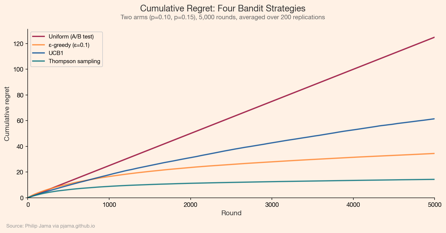
A good bandit algorithm has sublinear regret: the per-round regret shrinks toward zero as the algorithm learns. Thompson sampling achieves logarithmic regret, matching the theoretical lower bound (the Lai-Robbins bound) up to constant factors. In contrast, a fixed-horizon A/B test with equal allocation accumulates linear regret throughout its exploration phase.
Regret Curves: Bandits vs. A/B Test
The following simulation compares cumulative regret across four strategies: uniform random allocation (the A/B test baseline), epsilon-greedy (explore with fixed probability), UCB1 (upper confidence bound), and Thompson sampling.
Cumulative regret curves showing Thompson sampling and UCB1 outperforming uniform allocation Show Python source
import math
import random
import numpy as np
import matplotlib
matplotlib.use('Agg')
import matplotlib.pyplot as plt

FT_BG = '#FFF1E5'
FT_CLARET = '#990F3D'
FT_OXFORD = '#0F5499'
FT_TEAL = '#0D7680'
FT_MANDARIN = '#FF8833'

plt.rcParams.update({
    'figure.facecolor': FT_BG,
    'axes.facecolor': FT_BG,
    'savefig.facecolor': FT_BG,
    'font.family': 'sans-serif',
    'font.sans-serif': ['Helvetica Neue', 'Arial', 'sans-serif'],
    'axes.spines.top': False,
    'axes.spines.right': False,
})

true_rates = np.array([0.10, 0.15])
best_rate = true_rates.max()
gaps = best_rate - true_rates
K = len(true_rates)
T = 5000
REPS = 200

def run_uniform(reps, T):
    regret = np.zeros((reps, T))
    for rep in range(reps):
        for t in range(T):
            arm = t % K
            regret[rep, t] = gaps[arm]
    return np.cumsum(regret, axis=1).mean(axis=0)

def run_epsilon_greedy(reps, T, eps=0.1):
    regret = np.zeros((reps, T))
    for rep in range(reps):
        counts = np.zeros(K)
        totals = np.zeros(K)
        for t in range(T):
            if np.random.random() < eps or counts.min() == 0:
                arm = np.random.randint(K)
            else:
                arm = np.argmax(totals / np.maximum(counts, 1))
            reward = 1.0 if np.random.random() < true_rates[arm] else 0.0
            counts[arm] += 1
            totals[arm] += reward
            regret[rep, t] = gaps[arm]
    return np.cumsum(regret, axis=1).mean(axis=0)

def run_ucb1(reps, T):
    regret = np.zeros((reps, T))
    for rep in range(reps):
        counts = np.zeros(K)
        totals = np.zeros(K)
        for t in range(T):
            if t < K:
                arm = t
            else:
                ucbs = totals / counts + np.sqrt(2 * math.log(t) / counts)
                arm = np.argmax(ucbs)
            reward = 1.0 if np.random.random() < true_rates[arm] else 0.0
            counts[arm] += 1
            totals[arm] += reward
            regret[rep, t] = gaps[arm]
    return np.cumsum(regret, axis=1).mean(axis=0)

def run_thompson(reps, T):
    regret = np.zeros((reps, T))
    for rep in range(reps):
        alphas = np.ones(K)
        betas = np.ones(K)
        for t in range(T):
            samples = np.array([np.random.beta(alphas[k], betas[k]) for k in range(K)])
            arm = np.argmax(samples)
            reward = 1.0 if np.random.random() < true_rates[arm] else 0.0
            alphas[arm] += reward
            betas[arm] += (1 - reward)
            regret[rep, t] = gaps[arm]
    return np.cumsum(regret, axis=1).mean(axis=0)

uniform_regret = run_uniform(REPS, T)
eps_regret = run_epsilon_greedy(REPS, T)
ucb_regret = run_ucb1(REPS, T)
thompson_regret = run_thompson(REPS, T)

rounds = np.arange(1, T + 1)

fig, ax = plt.subplots(figsize=(10, 5))
ax.plot(rounds, uniform_regret, color=FT_CLARET, linewidth=2, label='Uniform (A/B test)', alpha=0.85)
ax.plot(rounds, eps_regret, color=FT_MANDARIN, linewidth=2, label='\u03b5-greedy (\u03b5=0.1)', alpha=0.85)
ax.plot(rounds, ucb_regret, color=FT_OXFORD, linewidth=2, label='UCB1', alpha=0.85)
ax.plot(rounds, thompson_regret, color=FT_TEAL, linewidth=2, label='Thompson sampling', alpha=0.85)

ax.set_xlim(0, T)
ax.set_ylim(0, None)
ax.set_xlabel('Round', fontsize=11, color='#333333')
ax.set_ylabel('Cumulative regret', fontsize=11, color='#333333')
ax.legend(fontsize=9, framealpha=0.9)

fig.text(0.5, 0.97, 'Cumulative Regret: Four Bandit Strategies',
         ha='center', fontsize=14, fontweight='bold', color='#333333')
fig.text(0.5, 0.935, 'Two arms (p=0.10, p=0.15), 5,000 rounds, averaged over 200 replications',
         ha='center', fontsize=10, color='#666666')
fig.text(0.02, 0.01, 'Source: Philip Jama via pjama.github.io',
         fontsize=8, color='#999999', ha='left')
fig.tight_layout(rect=[0, 0.03, 1, 0.92])
fig.savefig('regret_comparison.png', dpi=150, bbox_inches='tight')

print('wrote regret_comparison.png')
Regret Minimization vs. Hypothesis Testing
A/B tests and bandits optimize for different objectives. A/B tests aim for statistical inference: estimating the treatment effect with controlled error rates (Type I and Type II). Bandits aim for cumulative reward: minimizing regret over the entire allocation period.
This distinction matters. A bandit that shifts traffic aggressively toward one arm may reach lower regret but produce biased estimates of each arm's true rate, because the losing arm receives fewer observations. If the goal is to measure the effect precisely (for a journal paper, a regulatory filing, or a reusable model), a fixed-allocation A/B test with proper power analysis is the right tool. If the goal is to maximize total conversions during the experiment itself (ad serving, homepage optimization), bandits are the better fit.
Other Bandit Algorithms
Thompson sampling is not the only option:
Epsilon-greedy: exploit the best arm with probability 1 - epsilon, explore uniformly with probability epsilon. Simple but wasteful: it explores arms already known to be bad at the same rate as promising unknowns.
UCB1 (Upper Confidence Bound): play the arm with the highest upper confidence bound on its estimated reward. Deterministic and well-analyzed, but less flexible with complex reward models.
Bayesian UCB: like UCB1 but uses the posterior's quantile as the upper bound. Combines the structure of UCB with Bayesian updating.
Contextual bandits: the reward depends on user features (context). LinUCB and neural contextual bandits generalize the multi-armed setting to personalized allocation.
When to Use Bandits vs. A/B Tests
Bandits are well suited when:
The cost of assigning users to a losing variant is high (revenue, user experience).
The number of variants is large and most will be pruned quickly.
The primary goal is cumulative performance, not precise effect estimation.
The environment is non-stationary (reward rates drift over time).
A/B tests are preferable when:
Unbiased effect estimates are required for downstream decisions.
Regulatory or scientific standards demand controlled error rates.
The experiment is short and the cost of equal allocation is small.
Interaction effects, network effects, or interference make adaptive allocation risky.
Many production systems use a hybrid: run a short A/B test to validate the effect, then switch to bandit allocation for ongoing optimization.
Implementation Considerations
Deploying Thompson sampling in production introduces practical concerns:
Batching: in real systems, outcomes arrive in batches (hourly, daily), not one at a time. Batch Thompson sampling updates posteriors once per batch and samples a single allocation vector, trading off exploration granularity for engineering simplicity.
Delayed rewards: if the conversion event occurs days after assignment, the posterior lags behind reality. Use conservative priors and longer update windows.
Multiple metrics: when optimizing for one metric while guarding another, constrained Thompson sampling samples from the posterior of the primary metric and rejects allocations that violate guardrail thresholds.
Non-stationarity: if arm rewards shift over time, use a discounted or sliding-window posterior to downweight old observations.
Looking Ahead
Bandits assume you can randomize: you control which arm each user sees. The next article in this series tackles the harder problem. When randomization is impossible -- because of ethical constraints, organizational inertia, or the treatment already happened -- causal inference from observational data provides tools to estimate effects from non-experimental evidence.
Thompson sampling allocates traffic adaptively, but it does not answer a different question: what happens when you cannot randomize at all? Observational causal inference picks up where experimentation leaves off.