Philip Jama

Articles /Decision Science /Part 5

Causal Inference from Observational Data

Propensity scores, difference-in-differences, and what randomization buys you

Decision ScienceCausal InferenceObservational StudiesPython

Randomized experiments are the gold standard for causal claims. Part 1 (Online Experiments with a Bayesian Lens) showed why: random assignment ensures that treatment and control groups differ only in the treatment itself, so any observed difference in outcomes can be attributed to the intervention. But randomization is not always possible. Ethical constraints, organizational realities, or the simple fact that the intervention already happened can rule out a controlled experiment.

Causal inference from observational data is the set of methods for estimating treatment effects when you cannot control assignment. The core challenge: without randomization, treated and untreated groups may differ systematically. Any naive comparison confounds the treatment effect with pre-existing differences. Every method in this article attacks that confounding problem from a different angle.

What Randomization Buys You

In a randomized experiment, treatment assignment is independent of all covariates, observed and unobserved. This independence makes the average outcome difference an unbiased estimator of the causal effect. Remove randomization and that guarantee disappears.

Consider a company that rolled out a new onboarding flow to users who signed up on weekdays. Weekend users kept the old flow. Comparing conversion rates directly would confuse the effect of the new flow with any weekday-vs-weekend differences in user behavior. The treatment (new onboarding) is confounded with the covariate (day of week).

The Potential Outcomes Framework

The Rubin causal model defines the causal effect for unit i as Y_i(1) - Y_i(0): the difference between the outcome under treatment and the outcome under control. The fundamental problem of causal inference is that you only observe one of these two potential outcomes for each unit. The other is the counterfactual.

All observational methods try to construct a credible estimate of the missing counterfactual. They differ in what assumptions they require and how they construct comparison groups.

Propensity Score Methods

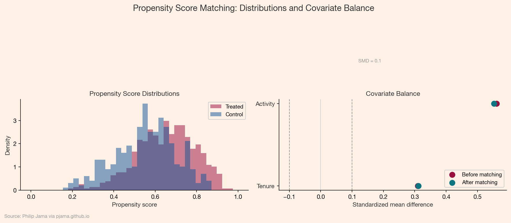
The propensity score is the probability of receiving treatment given observed covariates: e(X) = P(T=1 | X). Rosenbaum and Rubin (1983) showed that conditioning on the propensity score balances all observed covariates between treated and untreated groups, mimicking the balance that randomization would provide.

Two common approaches use the propensity score:

Propensity Score Matching

For each treated unit, find one or more untreated units with a similar propensity score. The matched pairs form a pseudo-randomized sample. The treatment effect estimate is the average outcome difference within matched pairs.

Matching works well when the propensity score distributions for treated and untreated groups overlap substantially. When overlap is poor (some treated units have no comparable controls), the method breaks down and honest reporting requires trimming those units.

Inverse Probability Weighting

Inverse probability weighting (IPW) reweights observations to create a pseudo-population where treatment assignment is independent of covariates. Treated units receive weight 1/e(X) and control units receive weight 1/(1-e(X)). The weighted average outcome difference estimates the average treatment effect.

IPW avoids discarding unmatched units but is sensitive to extreme propensity scores. When e(X) is close to 0 or 1, the weights explode and variance increases sharply. Stabilized weights and weight trimming mitigate this.

Propensity score distributions and covariate balance before and after matching
Show Python source
import math
import numpy as np
import matplotlib
matplotlib.use('Agg')
import matplotlib.pyplot as plt

np.random.seed(42)

FT_BG = '#FFF1E5'
FT_CLARET = '#990F3D'
FT_OXFORD = '#0F5499'
FT_TEAL = '#0D7680'

plt.rcParams.update({
    'figure.facecolor': FT_BG,
    'axes.facecolor': FT_BG,
    'savefig.facecolor': FT_BG,
    'font.family': 'sans-serif',
    'font.sans-serif': ['Helvetica Neue', 'Arial', 'sans-serif'],
    'axes.spines.top': False,
    'axes.spines.right': False,
})

# Generate synthetic observational data
n = 1000
tenure = np.random.normal(24, 12, n).clip(1, 72)
activity = np.random.normal(50, 20, n).clip(0, 100)

# Treatment assignment depends on confounders
log_odds = -2.0 + 0.04 * tenure + 0.03 * activity
p_treat = 1 / (1 + np.exp(-log_odds))
treatment = (np.random.rand(n) < p_treat).astype(float)

# Outcome with true effect = +2.0
outcome = 0.5 * tenure / 12 + 0.1 * activity + 2.0 * treatment + np.random.normal(0, 2, n)

# Logistic regression via gradient descent for propensity scores
tenure_z = (tenure - tenure.mean()) / tenure.std()
activity_z = (activity - activity.mean()) / activity.std()
X = np.column_stack([np.ones(n), tenure_z, activity_z])
theta = np.zeros(3)
for _ in range(1000):
    pred = 1 / (1 + np.exp(-X @ theta))
    grad = X.T @ (pred - treatment) / n
    theta -= 1.0 * grad
pscore = 1 / (1 + np.exp(-X @ theta))

# Nearest-neighbor matching without replacement
treated_idx = np.where(treatment == 1)[0]
control_idx = np.where(treatment == 0)[0]
matched_control = []
used = set()
for t in treated_idx:
    best_dist = float('inf')
    best_c = -1
    for c in control_idx:
        if c in used:
            continue
        d = abs(pscore[t] - pscore[c])
        if d < best_dist:
            best_dist = d
            best_c = c
    if best_c >= 0:
        matched_control.append(best_c)
        used.add(best_c)
matched_control = np.array(matched_control)
matched_treated = treated_idx[:len(matched_control)]

# Covariate balance: standardized mean difference
def smd(x_t, x_c):
    pooled_std = np.sqrt((x_t.var() + x_c.var()) / 2)
    if pooled_std == 0:
        return 0
    return (x_t.mean() - x_c.mean()) / pooled_std

covariates = ['Tenure', 'Activity']
raw_data = [tenure, activity]

smd_before = [smd(raw_data[i][treated_idx], raw_data[i][control_idx]) for i in range(2)]
smd_after = [smd(raw_data[i][matched_treated], raw_data[i][matched_control]) for i in range(2)]

# Plot
fig, (ax1, ax2) = plt.subplots(1, 2, figsize=(12, 5))

# Left: propensity score distributions
bins = np.linspace(0, 1, 40)
ax1.hist(pscore[treatment == 1], bins=bins, color=FT_CLARET, alpha=0.5, label='Treated', density=True)
ax1.hist(pscore[treatment == 0], bins=bins, color=FT_OXFORD, alpha=0.5, label='Control', density=True)
ax1.set_xlabel('Propensity score', fontsize=10, color='#333333')
ax1.set_ylabel('Density', fontsize=10, color='#333333')
ax1.legend(fontsize=9, framealpha=0.9)
ax1.set_title('Propensity Score Distributions', fontsize=11, color='#333333')

# Right: covariate balance
y_pos = np.arange(len(covariates))
ax2.scatter(smd_before, y_pos, color=FT_CLARET, s=80, zorder=3, label='Before matching')
ax2.scatter(smd_after, y_pos, color=FT_TEAL, s=80, zorder=3, label='After matching')
for i in range(len(covariates)):
    ax2.plot([smd_before[i], smd_after[i]], [y_pos[i], y_pos[i]],
             color='#999999', linewidth=1.5, zorder=2)
ax2.axvline(x=0.1, color='#999999', linewidth=1, linestyle='--')
ax2.axvline(x=-0.1, color='#999999', linewidth=1, linestyle='--')
ax2.axvline(x=0, color='#cccccc', linewidth=0.8)
ax2.text(0.12, len(covariates) - 0.5, 'SMD = 0.1', fontsize=8, color='#999999')
ax2.set_yticks(y_pos)
ax2.set_yticklabels(covariates, fontsize=10, color='#333333')
ax2.set_xlabel('Standardized mean difference', fontsize=10, color='#333333')
ax2.legend(fontsize=9, framealpha=0.9, loc='lower right')
ax2.set_title('Covariate Balance', fontsize=11, color='#333333')

fig.text(0.5, 0.97, 'Propensity Score Matching: Distributions and Covariate Balance',
         ha='center', fontsize=14, fontweight='bold', color='#333333')
fig.text(0.02, 0.01, 'Source: Philip Jama via pjama.github.io',
         fontsize=8, color='#999999', ha='left')
fig.tight_layout(rect=[0, 0.03, 1, 0.92])
fig.savefig('propensity_matching.png', dpi=150, bbox_inches='tight')

print('wrote propensity_matching.png')

Difference-in-Differences

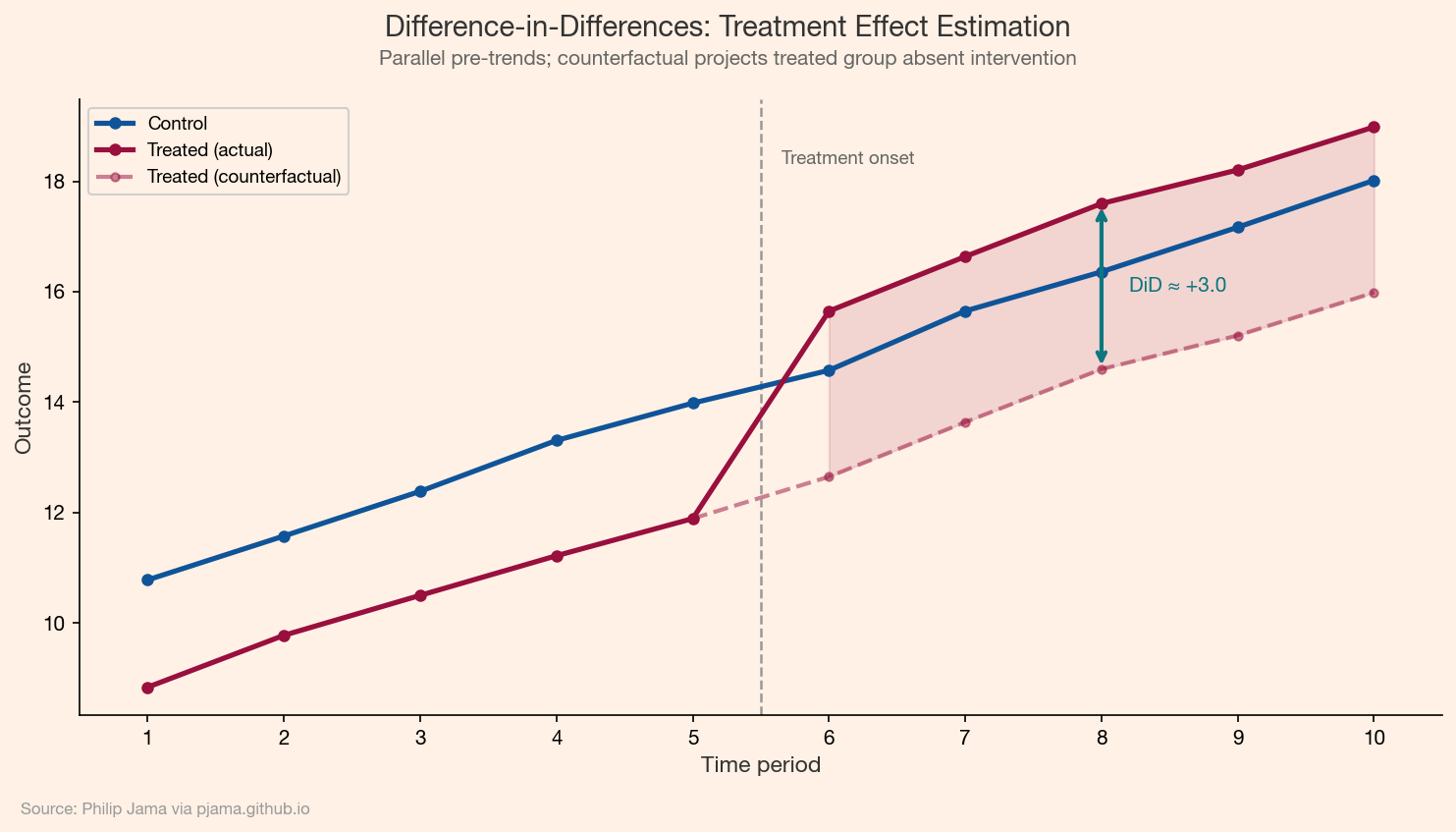
Difference-in-differences (DiD) exploits a natural experiment where treatment timing varies across groups. The method compares the change in outcomes before and after treatment for the treated group against the same change for the control group. The "double difference" removes time-invariant confounders (group-level) and common time trends (period-level).

The identifying assumption is parallel trends: absent the treatment, the treated and control groups would have followed the same trajectory. This assumption is untestable in the post-treatment period, but you can check whether pre-treatment trends are parallel as a plausibility diagnostic.

Difference-in-differences: treated and control trajectories with counterfactual
Show Python source
import random
import matplotlib
matplotlib.use('Agg')
import matplotlib.pyplot as plt

random.seed(42)

FT_BG = '#FFF1E5'
FT_CLARET = '#990F3D'
FT_OXFORD = '#0F5499'
FT_TEAL = '#0D7680'

plt.rcParams.update({
    'figure.facecolor': FT_BG,
    'axes.facecolor': FT_BG,
    'savefig.facecolor': FT_BG,
    'font.family': 'sans-serif',
    'font.sans-serif': ['Helvetica Neue', 'Arial', 'sans-serif'],
    'axes.spines.top': False,
    'axes.spines.right': False,
})

periods = list(range(1, 11))
treat_onset = 5.5
effect = 3.0

# Parallel pre-trends with slight noise
control = [10 + 0.8 * t + random.gauss(0, 0.15) for t in periods]
treated_base = [8 + 0.8 * t + random.gauss(0, 0.15) for t in periods]
treated_actual = [treated_base[i] + (effect if t >= 6 else 0) for i, t in enumerate(periods)]
counterfactual = treated_base[:]

fig, ax = plt.subplots(figsize=(10, 5.5))

# Control and treated lines
ax.plot(periods, control, color=FT_OXFORD, linewidth=2.5, marker='o', markersize=5,
        label='Control', zorder=3)
ax.plot(periods, treated_actual, color=FT_CLARET, linewidth=2.5, marker='o', markersize=5,
        label='Treated (actual)', zorder=3)

# Counterfactual from period 5 onward
cf_periods = [p for p in periods if p >= 5]
cf_values = [counterfactual[i] for i, p in enumerate(periods) if p >= 5]
ax.plot(cf_periods, cf_values, color=FT_CLARET, linewidth=2, linestyle='--', alpha=0.5,
        marker='o', markersize=4, label='Treated (counterfactual)', zorder=2)

# Shade treatment effect
post_periods = [p for p in periods if p >= 6]
post_actual = [treated_actual[i] for i, p in enumerate(periods) if p >= 6]
post_cf = [counterfactual[i] for i, p in enumerate(periods) if p >= 6]
ax.fill_between(post_periods, post_actual, post_cf, color=FT_CLARET, alpha=0.12)

# Treatment onset line
ax.axvline(x=treat_onset, color='#999999', linewidth=1.2, linestyle='--')
ax.text(treat_onset + 0.15, max(control) + 0.3, 'Treatment onset', fontsize=9,
        color='#666666', rotation=0)

# DiD annotation arrow at period 8
idx8 = 7
ax.annotate('', xy=(8, treated_actual[idx8]), xytext=(8, counterfactual[idx8]),
            arrowprops=dict(arrowstyle='<->', color=FT_TEAL, lw=2))
mid_y = (treated_actual[idx8] + counterfactual[idx8]) / 2
ax.text(8.2, mid_y, f'DiD \u2248 +{effect:.1f}', fontsize=10, fontweight='bold',
        color=FT_TEAL, va='center')

ax.set_xlim(0.5, 10.5)
ax.set_xlabel('Time period', fontsize=11, color='#333333')
ax.set_ylabel('Outcome', fontsize=11, color='#333333')
ax.set_xticks(periods)
ax.legend(fontsize=9, framealpha=0.9, loc='upper left')

fig.text(0.5, 0.97, 'Difference-in-Differences: Treatment Effect Estimation',
         ha='center', fontsize=14, fontweight='bold', color='#333333')
fig.text(0.5, 0.935, 'Parallel pre-trends; counterfactual projects treated group absent intervention',
         ha='center', fontsize=10, color='#666666')
fig.text(0.02, 0.01, 'Source: Philip Jama via pjama.github.io',
         fontsize=8, color='#999999', ha='left')
fig.tight_layout(rect=[0, 0.03, 1, 0.92])
fig.savefig('did_visualization.png', dpi=150, bbox_inches='tight')

print('wrote did_visualization.png')

Instrumental Variables

When unobserved confounders bias the treatment effect, an instrumental variable (IV) can recover a causal estimate. An instrument Z must satisfy three conditions:

  1. Relevance: Z is correlated with the treatment.
  2. Exclusion: Z affects the outcome only through the treatment.
  3. Independence: Z is independent of unobserved confounders.

The classic example: distance to a college as an instrument for years of education when estimating the effect of education on earnings. Distance affects whether someone attends college but (arguably) does not directly affect earnings.

The IV estimator uses two-stage least squares. In the first stage, regress treatment on the instrument. In the second stage, regress the outcome on the predicted treatment values. The resulting coefficient estimates the local average treatment effect (LATE): the causal effect for the subpopulation whose treatment status is influenced by the instrument.

Causal Graphs and the DAG Framework

All of these methods benefit from thinking in terms of directed acyclic graphs (DAGs). A DAG encodes assumptions about which variables cause which others. Given a DAG, you can read off which variables to condition on (the adjustment set) and which to leave alone.

The connection to graph analysis runs deep. Part 9 of the Network Graph Analysis series covers DAGs, d-separation, and do-calculus in detail. The key principle here: conditioning on a collider (a variable caused by both treatment and outcome) introduces bias rather than removing it. Drawing the DAG before choosing a method prevents this mistake.

Choosing a Method

The right method depends on what you can assume:

Method Key Assumption Handles Unobserved Confounders?
Propensity score matching Selection on observables No
Inverse probability weighting Selection on observables No
Difference-in-differences Parallel trends Time-invariant ones
Instrumental variables Valid instrument exists Yes (for compliers)

No method is assumption-free. The honest practice is to state the identifying assumption, assess its plausibility, and run sensitivity analyses to check how fragile the estimate is to violations.

Looking Ahead

Observational methods estimate effects when the experiment is already over. A different practical challenge arises when the experiment is still running: how to monitor accumulating evidence and decide when enough data has arrived. Sequential testing and early stopping provides the formal machinery, connecting the Bayesian posterior monitoring introduced in Part 2 (Bayesian Sample Efficiency) with rigorous stopping rules.

Observational methods estimate effects after the fact. A complementary problem arises during an experiment: when should you stop collecting data and declare a result? Sequential testing formalizes early stopping.

View all articles in Decision Science

Collaborate

If you're exploring related work and need hands-on help, I'm open to consulting and advisory. Get in touch