Philip Jama

Articles /Network Graph Analysis /Part 4

Building Knowledge Graphs from Text

From raw text to structured concept networks

Knowledge GraphsNLPPythonNetwork Analysis

Text is full of implicit structure: entities, relationships, hierarchies that a knowledge graph makes explicit. By extracting concepts and their connections from documents, we transform unstructured prose into a navigable network of ideas. This article covers the pipeline from text to graph, drawing on the concept extraction and associative network techniques used in the Graphception project ↗.

What Is a Knowledge Graph

A knowledge graph represents information as a network of entities (nodes) connected by labeled relationships (edges). Unlike a flat database table, a knowledge graph captures the structure of knowledge: how concepts relate, which ideas are central, and where clusters of related topics form. Examples range from Wikidata and Google’s Knowledge Graph to domain-specific ontologies in medicine, law, and engineering.

Entity and Relation Extraction

The first step is pulling structured triples (subject, relation, object) from text. Approaches range from rule-based (dependency parsing + patterns) to statistical (named entity recognition + relation classification) to neural (end-to-end transformer models). The choice depends on domain, corpus size, and required precision.

Co-occurrence Networks vs. Semantic Graphs

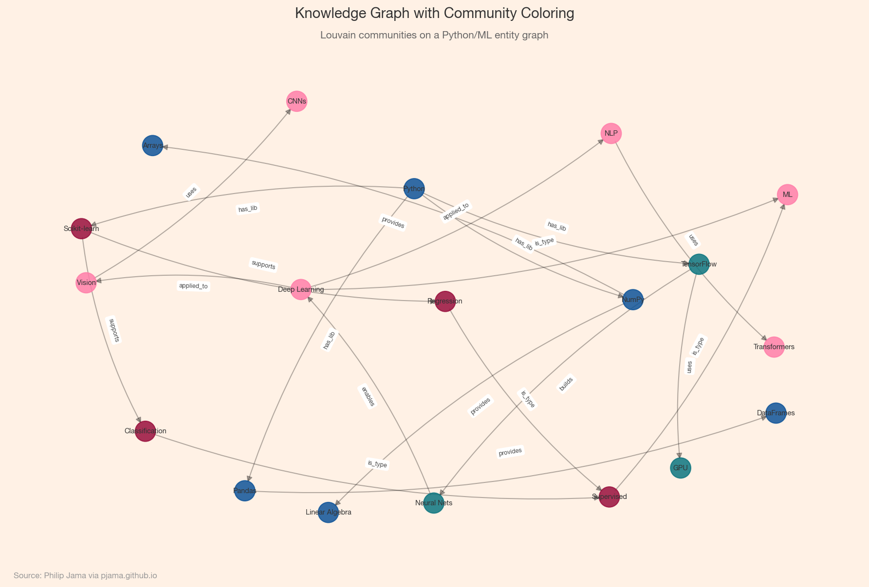
The simplest knowledge graph is a co-occurrence network: two concepts share an edge if they appear together (in a sentence, paragraph, or document). This captures topical association but not the type of relationship. A semantic graph adds labeled, directed edges (e.g., causes, part-of, treats) that encode meaning. Co-occurrence networks are easy to build; semantic graphs require deeper NLP but yield richer reasoning.

Co-occurrence knowledge graph extracted from text with sized nodes
Show Python source
import networkx as nx
import numpy as np
import matplotlib
matplotlib.use('Agg')
import matplotlib.pyplot as plt
from matplotlib.colors import LinearSegmentedColormap
from collections import Counter

FT_BG = '#FFF1E5'
FT_CLARET = '#990F3D'
FT_OXFORD = '#0F5499'
FT_TEAL = '#0D7680'

plt.rcParams.update({
    'figure.facecolor': FT_BG,
    'axes.facecolor': FT_BG,
    'savefig.facecolor': FT_BG,
    'font.family': 'sans-serif',
    'font.sans-serif': ['Helvetica Neue', 'Arial', 'sans-serif'],
    'axes.spines.top': False,
    'axes.spines.right': False,
})

np.random.seed(42)

corpus = [
    'Neural networks learn representations from data using backpropagation.',
    'Deep learning extends neural networks with multiple hidden layers.',
    'Backpropagation computes gradients for training deep learning models.',
    'Convolutional networks excel at image recognition and computer vision.',
    'Recurrent networks handle sequential data like text and time series.'
]

concepts = ['neural networks', 'deep learning', 'backpropagation', 'representations',
            'data', 'hidden layers', 'gradients', 'training', 'models',
            'convolutional networks', 'image recognition', 'computer vision',
            'recurrent networks', 'sequential data', 'text', 'time series']

freq = Counter()
G = nx.Graph()
for sent in corpus:
    lower = sent.lower()
    present = [c for c in concepts if c in lower]
    for c in present:
        freq[c] += 1
    for i, c1 in enumerate(present):
        for c2 in present[i+1:]:
            if G.has_edge(c1, c2):
                G[c1][c2]['weight'] += 1
            else:
                G.add_edge(c1, c2, weight=1)

for n in G.nodes():
    if n not in freq:
        freq[n] = 1

sizes = [freq[n] * 600 + 200 for n in G.nodes()]

ft_cmap = LinearSegmentedColormap.from_list('ft', [FT_OXFORD, FT_TEAL, FT_CLARET])

fig, ax = plt.subplots(figsize=(10, 7))
pos = nx.spring_layout(G, seed=42, k=2)
nx.draw_networkx_edges(G, pos, ax=ax, alpha=0.3, width=1.5)
nx.draw_networkx_nodes(G, pos, ax=ax, node_size=sizes,
                       node_color=list(range(len(G))),
                       cmap=ft_cmap, alpha=0.85)
nx.draw_networkx_labels(G, pos, ax=ax, font_size=8, font_color='#333333')
ax.set_axis_off()

fig.text(0.5, 0.97, 'Concept Co-occurrence Graph from ML Corpus',
         ha='center', fontsize=14, fontweight='bold', color='#333333')
fig.text(0.5, 0.935, 'Node size proportional to term frequency',
         ha='center', fontsize=10, color='#666666')
fig.text(0.02, 0.01, 'Source: Philip Jama via pjama.github.io',
         fontsize=8, color='#999999', ha='left')
fig.tight_layout(rect=[0, 0.03, 1, 0.92])
fig.savefig('concept_cooccurrence.png', dpi=150, bbox_inches='tight')

print('wrote concept_cooccurrence.png')

Community Structure in Concept Networks

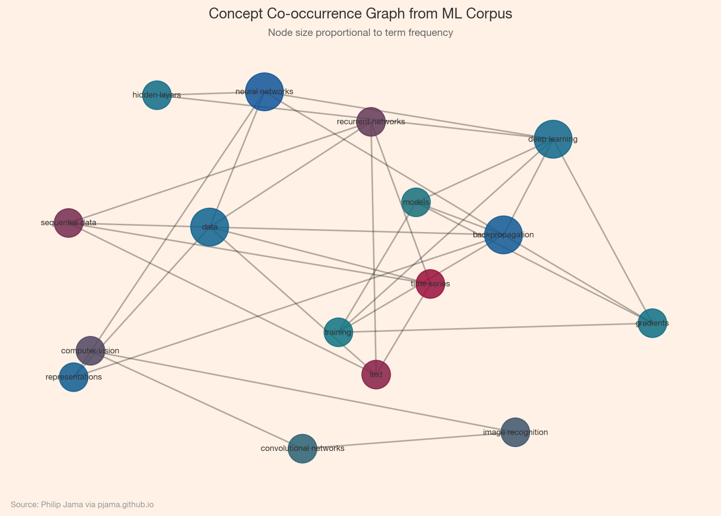
Once you have a concept graph, community detection (Part 2) reveals topic clusters: groups of concepts that co-occur frequently. These clusters often correspond to subtopics or themes within the corpus. Visualizing them helps identify the main threads in a body of text and the bridging concepts that connect different domains. The Graphception project ↗ demonstrates this pipeline on real text corpora.

Semantic knowledge graph with community coloring and labeled edges
Show Python source
import networkx as nx
import numpy as np
import matplotlib
matplotlib.use('Agg')
import matplotlib.pyplot as plt

FT_BG = '#FFF1E5'
FT_CLARET = '#990F3D'
FT_OXFORD = '#0F5499'
FT_TEAL = '#0D7680'
FT_CANDY = '#FF7FAA'

plt.rcParams.update({
    'figure.facecolor': FT_BG,
    'axes.facecolor': FT_BG,
    'savefig.facecolor': FT_BG,
    'font.family': 'sans-serif',
    'font.sans-serif': ['Helvetica Neue', 'Arial', 'sans-serif'],
    'axes.spines.top': False,
    'axes.spines.right': False,
})

np.random.seed(42)

G = nx.DiGraph()
edges = [
    ('Python', 'NumPy', 'has_lib'), ('Python', 'Pandas', 'has_lib'),
    ('Python', 'Scikit-learn', 'has_lib'), ('Python', 'TensorFlow', 'has_lib'),
    ('NumPy', 'Arrays', 'provides'), ('Pandas', 'DataFrames', 'provides'),
    ('Scikit-learn', 'Classification', 'supports'), ('Scikit-learn', 'Regression', 'supports'),
    ('TensorFlow', 'Neural Nets', 'builds'), ('TensorFlow', 'GPU', 'uses'),
    ('Neural Nets', 'Deep Learning', 'enables'), ('Deep Learning', 'NLP', 'applied_to'),
    ('Deep Learning', 'Vision', 'applied_to'), ('Classification', 'Supervised', 'is_type'),
    ('Regression', 'Supervised', 'is_type'), ('NLP', 'Transformers', 'uses'),
    ('Vision', 'CNNs', 'uses'), ('Supervised', 'ML', 'is_type'),
    ('Deep Learning', 'ML', 'is_type'), ('NumPy', 'Linear Algebra', 'provides')
]
for u, v, r in edges:
    G.add_edge(u, v, relation=r)

Gu = G.to_undirected()
comms = nx.community.louvain_communities(Gu, seed=42)
ft_palette = [FT_OXFORD, FT_CLARET, FT_TEAL, FT_CANDY]
node_color_map = {}
for i, comm in enumerate(comms):
    for n in comm:
        node_color_map[n] = ft_palette[i % len(ft_palette)]

fig, ax = plt.subplots(figsize=(12, 8))
pos = nx.spring_layout(G, seed=42, k=1.8)
colors = [node_color_map.get(n, '#999') for n in G.nodes()]
nx.draw_networkx_edges(G, pos, ax=ax, alpha=0.3, width=1, arrows=True,
                       arrowsize=12, connectionstyle='arc3,rad=0.1')
nx.draw_networkx_nodes(G, pos, ax=ax, node_color=colors,
                       node_size=400, alpha=0.85)
nx.draw_networkx_labels(G, pos, ax=ax, font_size=7, font_color='#333333')
edge_labels = {(u, v): d['relation'] for u, v, d in G.edges(data=True)}
nx.draw_networkx_edge_labels(G, pos, edge_labels, ax=ax, font_size=6, alpha=0.7)
ax.set_axis_off()

fig.text(0.5, 0.97, 'Knowledge Graph with Community Coloring',
         ha='center', fontsize=14, fontweight='bold', color='#333333')
fig.text(0.5, 0.935, 'Louvain communities on a Python/ML entity graph',
         ha='center', fontsize=10, color='#666666')
fig.text(0.02, 0.01, 'Source: Philip Jama via pjama.github.io',
         fontsize=8, color='#999999', ha='left')
fig.tight_layout(rect=[0, 0.03, 1, 0.92])
fig.savefig('knowledge_graph_communities.png', dpi=150, bbox_inches='tight')

print('wrote knowledge_graph_communities.png')

Scaling and Storage Considerations

Small knowledge graphs fit in memory as NetworkX objects. Larger graphs benefit from graph databases (Neo4j, Amazon Neptune) or RDF triple stores (Apache Jena). For analysis at scale, adjacency-list formats (edge lists, CSR matrices) and distributed frameworks (GraphX, DGL) keep things tractable. The choice of storage shapes what queries are efficient: traversals, pattern matching, or bulk analytics.

Co-occurrence and NLP pipelines produce structured graphs, but they miss implicit relations. Large language models can fill those gaps.

View all articles in Network Graph Analysis

Collaborate

If you're exploring related work and need hands-on help, I'm open to consulting and advisory. Get in touch