Philip Jama

Articles /Decision Science /Part 3

The Secretary Problem and Optimal Stopping

When to stop looking and commit: the 37% rule and beyond

Decision ScienceOptimal StoppingProbabilityPython

You're hiring for a critical role. Candidates arrive one at a time, you can rank them against those you've already seen, but once you reject someone they're gone forever. How do you maximize your chance of picking the best? This is the secretary problem: one of the most elegant results in probability and decision theory. The optimal strategy is surprisingly simple: observe the first ~37% of candidates without hiring anyone, then immediately hire the next candidate who is better than all those you've seen.

The Classic Setup

The problem has clean assumptions:

  • There are n candidates, arriving in random order.
  • After each interview, you can rank the current candidate relative to all previous ones.
  • You must accept or reject each candidate immediately: no callbacks.
  • Your goal is to select the single best candidate (not just a good one).

Under these rules, a naive strategy (pick randomly) gives you a 1/n chance of getting the best. The optimal strategy does dramatically better.

The 1/e Rule: Why 37%?

The optimal strategy is a look-then-leap rule:

  1. Look phase: Interview the first r candidates and reject them all, but track the best score seen.
  2. Leap phase: From candidate r+1 onward, hire the first person who beats every candidate in the look phase.

The optimal cutoff r is approximately n/e (where e ≈ 2.718), which means you should observe about 37% of the pool before switching to selection mode. With this strategy, you select the best candidate with probability ~1/e ≈ 0.368 -- regardless of how large n is. That's a striking result: even with 1,000 candidates, you have a 37% chance of picking the absolute best by using this simple rule.

Success probability vs look-phase cutoff showing the 1/e optimum
Show Python source
import math
import random
import matplotlib
matplotlib.use('Agg')
import matplotlib.pyplot as plt

random.seed(42)

FT_BG = '#FFF1E5'
FT_CLARET = '#990F3D'
FT_OXFORD = '#0F5499'
FT_TEAL = '#0D7680'
FT_MANDARIN = '#FF8833'

plt.rcParams.update({
    'figure.facecolor': FT_BG,
    'axes.facecolor': FT_BG,
    'savefig.facecolor': FT_BG,
    'font.family': 'sans-serif',
    'font.sans-serif': ['Helvetica Neue', 'Arial', 'sans-serif'],
    'axes.spines.top': False,
    'axes.spines.right': False,
})

def simulate_secretary(n, cutoff_frac, trials):
    successes = 0
    k = max(1, int(cutoff_frac * n))
    for _ in range(trials):
        candidates = list(range(n))
        random.shuffle(candidates)
        best_in_look = max(candidates[:k]) if k > 0 else -1
        selected = None
        for c in candidates[k:]:
            if c > best_in_look:
                selected = c
                break
        if selected == n - 1:
            successes += 1
    return successes / trials

configs = [
    (10, 5000, FT_OXFORD, 'n = 10'),
    (50, 3000, FT_TEAL, 'n = 50'),
    (200, 2000, FT_CLARET, 'n = 200'),
    (1000, 800, FT_MANDARIN, 'n = 1,000'),
]

fracs = [i / 50 for i in range(1, 50)]

fig, ax = plt.subplots(figsize=(9, 5))

for n, trials, color, label in configs:
    probs = [simulate_secretary(n, r, trials) for r in fracs]
    ax.plot(fracs, probs, color=color, linewidth=2, label=label, alpha=0.85)

inv_e = 1 / math.e
ax.axhline(y=inv_e, color='#999999', linewidth=1.2, linestyle='--')
ax.axvline(x=inv_e, color='#999999', linewidth=1.2, linestyle='--')
ax.text(0.72, inv_e + 0.012, f'1/e \u2248 {inv_e:.3f}', fontsize=10, color='#666666')

ax.set_xlim(0, 1)
ax.set_ylim(0, 0.5)
ax.set_xlabel('Look-phase cutoff fraction (r)', fontsize=11, color='#333333')
ax.set_ylabel('Success probability', fontsize=11, color='#333333')
ax.legend(fontsize=9, framealpha=0.9)

fig.text(0.5, 0.97, 'Secretary Problem: Optimal Look-Phase Cutoff',
         ha='center', fontsize=14, fontweight='bold', color='#333333')
fig.text(0.5, 0.935, 'Success probability by cutoff fraction for different pool sizes',
         ha='center', fontsize=10, color='#666666')
fig.text(0.02, 0.01, 'Source: Philip Jama via pjama.github.io',
         fontsize=8, color='#999999', ha='left')
fig.tight_layout(rect=[0, 0.03, 1, 0.92])
fig.savefig('secretary_simulation.png', dpi=150, bbox_inches='tight')

print('wrote secretary_simulation.png')

Intuition Behind the Proof

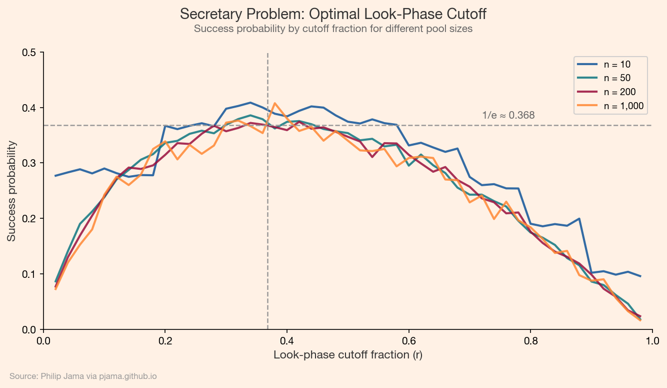
For a given cutoff r, the probability of selecting the best candidate can be written as a sum: for each position i > r, the best candidate is at position i and the best of the first i-1 candidates falls in the look phase (positions 1 through r). This leads to:

$$P(\text{win} \mid r) = \frac{r}{n} \sum_{i=r+1}^{n} \frac{1}{i-1}$$

As $n \to \infty$, this sum approximates $-\frac{r}{n} \ln!\left(\frac{r}{n}\right)$. Maximizing over the ratio $r/n$ gives the optimal fraction $1/e$, and the maximum probability converges to $1/e$.

Real-World Applications

The secretary problem isn't just a mathematical curiosity -- it maps onto many sequential decision problems:

  • Hiring: Interviewing candidates for a role where you must decide on the spot.
  • House hunting: Viewing apartments or houses in a competitive market where offers must be immediate.
  • Parking: Driving past open spots, deciding when to commit vs. keep looking for something closer.
  • A/B test variants: Running sequential experiments where each variant costs traffic. Observe early results to calibrate expectations, then commit when a candidate outperforms the baseline by enough to act on.

In each case, the core tension is the same: explore too little and you miss better options; explore too long and the best options are gone.

Variants and Extensions

The classic problem has spawned a rich family of variants:

  • Unknown n: When you don't know how many candidates exist, the strategy adapts using a time-based cutoff.
  • Multiple choices: If you can hire k candidates instead of one, the optimal look phase shrinks.
  • Partial information: If you can see cardinal scores (not just rankings), threshold-based strategies can outperform the 1/e rule.
  • Cost of search: When each interview has a cost, the optimal strategy becomes more aggressive: you stop earlier because continued search has diminishing returns.
  • Satisficing: Herbert Simon's alternative: set an acceptability threshold and take the first candidate who clears it, rather than maximizing.
Comparison of success rates across secretary problem variants
Show Python source
import math
import random
import matplotlib
matplotlib.use('Agg')
import matplotlib.pyplot as plt

random.seed(42)

FT_BG = '#FFF1E5'
FT_CLARET = '#990F3D'
FT_OXFORD = '#0F5499'
FT_TEAL = '#0D7680'
FT_CANDY = '#FF7FAA'
FT_MANDARIN = '#FF8833'

plt.rcParams.update({
    'figure.facecolor': FT_BG,
    'axes.facecolor': FT_BG,
    'savefig.facecolor': FT_BG,
    'font.family': 'sans-serif',
    'font.sans-serif': ['Helvetica Neue', 'Arial', 'sans-serif'],
    'axes.spines.top': False,
    'axes.spines.right': False,
})

TRIALS = 5000
N = 100

def classic_secretary(n, trials):
    k = max(1, int(n / math.e))
    wins = 0
    for _ in range(trials):
        c = list(range(n))
        random.shuffle(c)
        best_look = max(c[:k]) if k > 0 else -1
        for x in c[k:]:
            if x > best_look:
                if x == n - 1:
                    wins += 1
                break
    return wins / trials

def unknown_n(trials):
    wins = 0
    for _ in range(trials):
        n = random.randint(10, 200)
        k = max(1, int(n / math.e))
        c = list(range(n))
        random.shuffle(c)
        best_look = max(c[:k]) if k > 0 else -1
        for x in c[k:]:
            if x > best_look:
                if x == n - 1:
                    wins += 1
                break
    return wins / trials

def multiple_choice(n, picks, trials):
    k = max(1, int(n / math.e))
    wins = 0
    for _ in range(trials):
        c = list(range(n))
        random.shuffle(c)
        best_look = max(c[:k]) if k > 0 else -1
        selected = []
        for x in c[k:]:
            if x > best_look:
                selected.append(x)
                if len(selected) == picks:
                    break
        if n - 1 in selected:
            wins += 1
    return wins / trials

def cost_of_search(n, cost_per_look, trials):
    k = max(1, int(n / math.e))
    wins = 0
    for _ in range(trials):
        c = list(range(n))
        random.shuffle(c)
        best_look = max(c[:k]) if k > 0 else -1
        found = False
        for idx, x in enumerate(c[k:], start=k):
            if x > best_look:
                payoff = x / (n - 1) - cost_per_look * idx
                if payoff > 0 and x == n - 1:
                    wins += 1
                found = True
                break
        if not found:
            pass
    return wins / trials

def satisficing(n, threshold_frac, trials):
    wins = 0
    threshold = int(n * threshold_frac)
    k = max(1, int(n / math.e))
    for _ in range(trials):
        c = list(range(n))
        random.shuffle(c)
        for x in c[k:]:
            if x >= threshold:
                if x == n - 1:
                    wins += 1
                break
    return wins / trials

results = [
    ('Classic (1/e rule)', classic_secretary(N, TRIALS), FT_OXFORD),
    ('Unknown n', unknown_n(TRIALS), FT_TEAL),
    ('Multiple choice (k=3)', multiple_choice(N, 3, TRIALS), FT_CLARET),
    ('Cost of search', cost_of_search(N, 0.005, TRIALS), FT_MANDARIN),
    ('Satisficing (top 10%)', satisficing(N, 0.9, TRIALS), FT_CANDY),
]

labels = [r[0] for r in results]
values = [r[1] for r in results]
colors = [r[2] for r in results]

fig, ax = plt.subplots(figsize=(9, 5))

y_pos = range(len(labels))
bars = ax.barh(y_pos, values, color=colors, alpha=0.85, height=0.6)

for bar, val in zip(bars, values):
    ax.text(bar.get_width() + 0.008, bar.get_y() + bar.get_height() / 2,
            f'{val:.3f}', va='center', fontsize=10, color='#333333')

ax.axvline(x=1/math.e, color='#999999', linewidth=1.2, linestyle='--')
ax.text(1/math.e + 0.008, len(labels) - 0.3, f'1/e \u2248 {1/math.e:.3f}',
        fontsize=9, color='#666666')

ax.set_yticks(y_pos)
ax.set_yticklabels(labels, fontsize=10, color='#333333')
ax.set_xlim(0, max(values) * 1.25)
ax.set_xlabel('Success probability', fontsize=11, color='#333333')
ax.invert_yaxis()

fig.text(0.5, 0.97, 'Secretary Problem Variants: Success Rate Comparison',
         ha='center', fontsize=14, fontweight='bold', color='#333333')
fig.text(0.5, 0.935, 'Simulated success probability under different problem formulations',
         ha='center', fontsize=10, color='#666666')
fig.text(0.02, 0.01, 'Source: Philip Jama via pjama.github.io',
         fontsize=8, color='#999999', ha='left')
fig.tight_layout(rect=[0, 0.03, 1, 0.92])
fig.savefig('variant_comparison.png', dpi=150, bbox_inches='tight')

print('wrote variant_comparison.png')

Connection to Optimal Stopping Theory

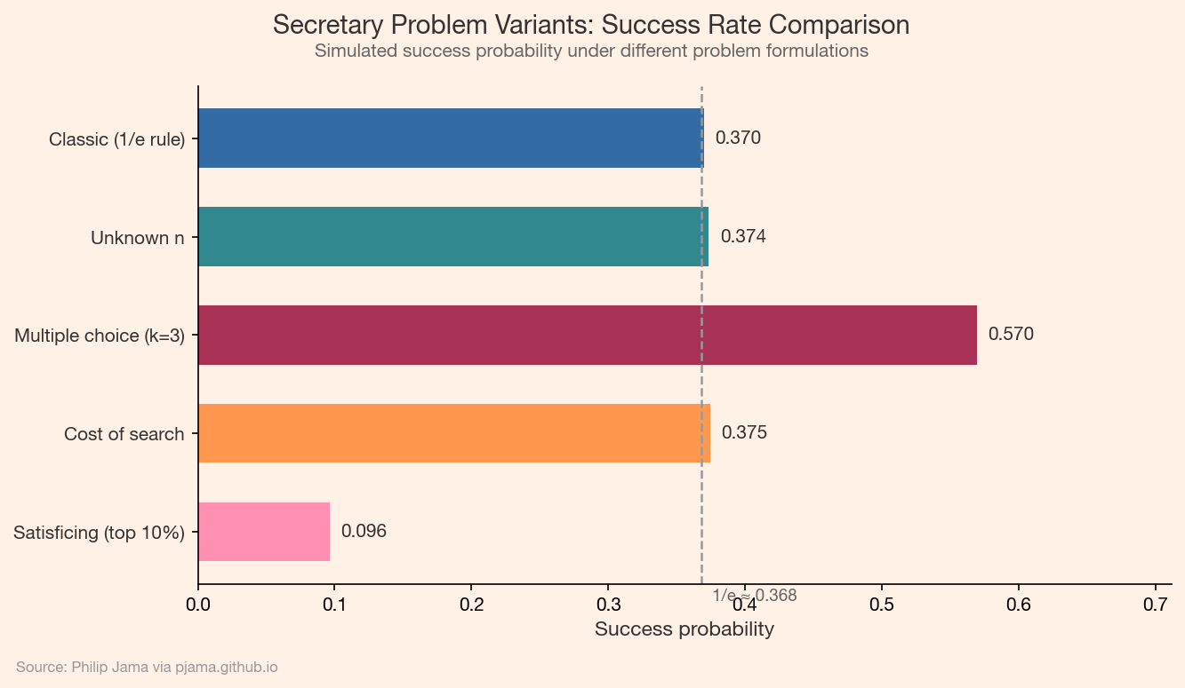
The secretary problem is the gateway to optimal stopping theory: the mathematics of deciding when to take an action to maximize reward. Related problems include:

  • The gambler's problem: When to cash out a sequence of gains.
  • Option pricing: The American option in finance is an optimal stopping problem.
  • Markov decision processes: Sequential decisions under uncertainty, where the Bayesian updating from Part 1 (Online Experiments with a Bayesian Lens) and Part 2 (Bayesian Sample Efficiency) connects naturally: each new observation updates your belief about whether you've found the best option.

Takeaway

The secretary problem teaches a deep lesson about the explore-exploit tradeoff: gathering information has value, but so does acting on it. The 37% rule gives a principled answer to "how long should you keep looking?" -- and the fact that it works regardless of the pool size makes it one of the most practically useful results in decision science.

The secretary problem shares the explore-exploit tension of Bayesian experimentation, but the mechanics differ: no priors, no posteriors, just ordinal rankings and an irrevocable accept-or-reject rule.

View all articles in Decision Science

Collaborate

If you're exploring related work and need hands-on help, I'm open to consulting and advisory. Get in touch