Graph Neural Networks: From Spectral to Spatial

Traditional neural networks assume grid-structured input: images are pixel grids, text is a token sequence. But many domains produce data that lives on irregular graphs: molecules, social networks, 3D meshes, knowledge bases. Graph Neural Networks (GNNs) extend deep learning to these structures, learning node and graph representations that capture both features and topology. This article covers the core architectures, from spectral graph convolutions to spatial message passing.

Why Deep Learning on Graphs

Hand-crafted graph features (degree, centrality, clustering) capture some structure but miss complex, task-specific patterns. GNNs learn features automatically from the graph, jointly encoding node attributes and neighborhood structure into dense embeddings useful for node classification, link prediction, and graph-level tasks.

Spectral Graph Convolutions

The spectral approach defines convolution via the graph Fourier transform (eigenvectors of the Laplacian, introduced in Part 3 (Centrality, Influence, and Spectral Methods)). Kipf & Welling’s Graph Convolutional Network (GCN) simplifies this to a single-hop neighborhood aggregation: each layer computes H’ = σ(Ã H W) where Ã is the normalized adjacency matrix with self-loops, H is the feature matrix, and W is a learnable weight matrix. Despite its simplicity, GCN is remarkably effective.

Spatial Methods and Message Passing

The message-passing framework generalizes GNNs: each node collects "messages" from its neighbors, aggregates them (sum, mean, max), and updates its own representation. Different architectures vary the message function, aggregation, and update rule. This spatial view is more flexible than spectral methods and naturally handles heterogeneous graphs and edge features.

Graph Attention Networks (GAT)

GAT replaces fixed aggregation weights (as in GCN) with learned attention coefficients. Each node attends to its neighbors with different weights, allowing the model to focus on the most relevant connections. Multi-head attention, borrowed from Transformers, provides stability and expressiveness. GAT often outperforms GCN on heterogeneous graphs where neighbors vary in relevance.

Show Python source

import numpy as np
import networkx as nx
import matplotlib
matplotlib.use('Agg')
import matplotlib.pyplot as plt
import random

FT_BG = '#FFF1E5'
FT_CLARET = '#990F3D'
FT_OXFORD = '#0F5499'
FT_TEAL = '#0D7680'
FT_MANDARIN = '#FF8833'

plt.rcParams.update({
    'figure.facecolor': FT_BG,
    'axes.facecolor': FT_BG,
    'savefig.facecolor': FT_BG,
    'font.family': 'sans-serif',
    'font.sans-serif': ['Helvetica Neue', 'Arial', 'sans-serif'],
    'axes.spines.top': False,
    'axes.spines.right': False,
})

random.seed(42)
np.random.seed(42)

# Synthetic citation network: 40 papers in 4 research topics
topics = ['NLP']*10 + ['Vision']*10 + ['Graphs']*10 + ['RL']*10
topic_colors = {'NLP': FT_OXFORD, 'Vision': FT_CLARET, 'Graphs': FT_TEAL, 'RL': FT_MANDARIN}
n = 40
G = nx.Graph()
for i in range(n):
    G.add_node(i, topic=topics[i])
for i in range(n):
    for j in range(i+1, n):
        p = 0.35 if topics[i] == topics[j] else 0.05
        if random.random() < p:
            G.add_edge(i, j)

labels = [0]*10 + [1]*10 + [2]*10 + [3]*10
A = nx.to_numpy_array(G)
A_hat = A + np.eye(n)
D_inv_sqrt = np.diag(1.0 / np.sqrt(A_hat.sum(axis=1)))
A_norm = D_inv_sqrt @ A_hat @ D_inv_sqrt

X = np.eye(n)
W1 = np.random.randn(n, 8) * 0.3
W2 = np.random.randn(8, 2) * 0.3
H1 = np.maximum(A_norm @ X @ W1, 0)
H2 = A_norm @ H1 @ W2

row_norms = np.sqrt((H2 ** 2).sum(axis=1, keepdims=True))
row_norms[row_norms == 0] = 1
cos_sim = (H2 @ H2.T) / (row_norms @ row_norms.T)
node_sim = cos_sim.mean(axis=1)
node_sim = (node_sim - node_sim.min()) / (node_sim.max() - node_sim.min() + 1e-8)

pos = nx.spring_layout(G, seed=42)
colors_gt = [topic_colors[topics[i]] for i in range(n)]

from matplotlib.colors import LinearSegmentedColormap
ft_cmap = LinearSegmentedColormap.from_list('ft', [FT_OXFORD, FT_TEAL, FT_CLARET])

fig, (ax1, ax2) = plt.subplots(1, 2, figsize=(14, 6))
nx.draw_networkx_edges(G, pos, ax=ax1, alpha=0.2, width=0.8)
nx.draw_networkx_nodes(G, pos, ax=ax1, node_color=colors_gt, node_size=200, alpha=0.85)
ax1.set_title('Ground Truth Topics', fontsize=12, color='#333333')
ax1.set_axis_off()
nx.draw_networkx_edges(G, pos, ax=ax2, alpha=0.2, width=0.8)
nx.draw_networkx_nodes(G, pos, ax=ax2, node_color=node_sim.tolist(),
                       cmap=ft_cmap, node_size=200, alpha=0.85)
ax2.set_title('GCN Embedding Similarity', fontsize=12, color='#333333')
ax2.set_axis_off()

fig.text(0.5, 0.97, '2-Layer GCN Forward Pass on Citation Network',
         ha='center', fontsize=14, fontweight='bold', color='#333333')
fig.text(0.02, 0.01, 'Source: Philip Jama via pjama.github.io',
         fontsize=8, color='#999999', ha='left')
fig.tight_layout(rect=[0, 0.03, 1, 0.92])
fig.savefig('gcn_karate.png', dpi=150, bbox_inches='tight')

print('wrote gcn_karate.png')

Node Classification Walkthrough

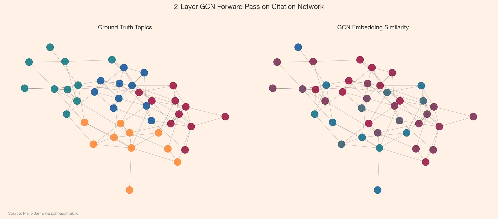
The canonical GNN task: given a graph where some nodes have known labels, predict the labels of the rest. The GCN or GAT learns embeddings that place same-class nodes nearby in representation space, then a final softmax layer classifies each node. The loss function -- cross-entropy -- is computed only on the labeled nodes, but message passing means every node's representation is shaped by its neighbors. Unlabeled nodes absorb information from labeled ones through the graph structure, so even a small labeled fraction can produce strong predictions across the entire graph.

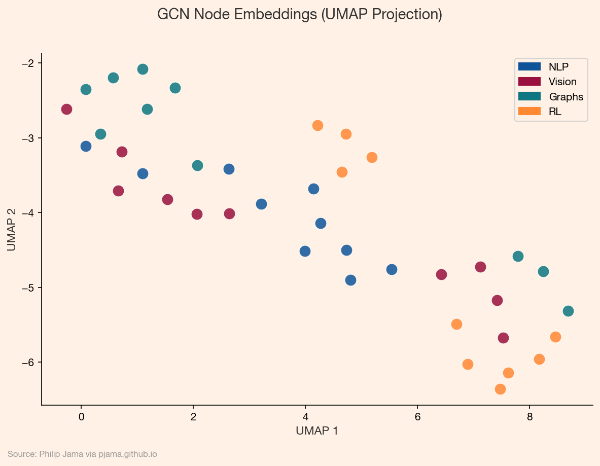
To see this in action, we can project the learned node embeddings into two dimensions using UMAP. Nodes that the GCN places close together in its high-dimensional embedding space should cluster by topic in the projection.

Show Python source

import numpy as np
import networkx as nx
import matplotlib
matplotlib.use('Agg')
import matplotlib.pyplot as plt
import umap
import random

FT_BG = '#FFF1E5'
FT_CLARET = '#990F3D'
FT_OXFORD = '#0F5499'
FT_TEAL = '#0D7680'
FT_MANDARIN = '#FF8833'

plt.rcParams.update({
    'figure.facecolor': FT_BG,
    'axes.facecolor': FT_BG,
    'savefig.facecolor': FT_BG,
    'font.family': 'sans-serif',
    'font.sans-serif': ['Helvetica Neue', 'Arial', 'sans-serif'],
    'axes.spines.top': False,
    'axes.spines.right': False,
})

random.seed(42)
np.random.seed(42)

# Same citation network as GCN forward pass
topics = ['NLP']*10 + ['Vision']*10 + ['Graphs']*10 + ['RL']*10
topic_colors = {'NLP': FT_OXFORD, 'Vision': FT_CLARET, 'Graphs': FT_TEAL, 'RL': FT_MANDARIN}
n = 40
G = nx.Graph()
for i in range(n):
    G.add_node(i, topic=topics[i])
for i in range(n):
    for j in range(i+1, n):
        p = 0.35 if topics[i] == topics[j] else 0.05
        if random.random() < p:
            G.add_edge(i, j)

A = nx.to_numpy_array(G)
A_hat = A + np.eye(n)
D_inv_sqrt = np.diag(1.0 / np.sqrt(A_hat.sum(axis=1)))
A_norm = D_inv_sqrt @ A_hat @ D_inv_sqrt

X = np.eye(n)
W1 = np.random.randn(n, 8) * 0.3
W2 = np.random.randn(8, 4) * 0.3
H1 = np.maximum(A_norm @ X @ W1, 0)
H2 = A_norm @ H1 @ W2

reducer = umap.UMAP(n_components=2, random_state=42, n_neighbors=8, min_dist=0.3)
proj = reducer.fit_transform(H2)

colors = [topic_colors[topics[i]] for i in range(n)]

fig, ax = plt.subplots(figsize=(8, 6))
for i, (x, y) in enumerate(proj):
    ax.scatter(x, y, c=colors[i], s=120, alpha=0.85, edgecolors='white', linewidth=0.5)
ax.set_xlabel('UMAP 1', fontsize=11, color='#333333')
ax.set_ylabel('UMAP 2', fontsize=11, color='#333333')
from matplotlib.patches import Patch
ax.legend(handles=[Patch(color=c, label=t) for t, c in topic_colors.items()], loc='best')

fig.text(0.5, 0.97, 'GCN Node Embeddings (UMAP Projection)',
         ha='center', fontsize=14, fontweight='bold', color='#333333')
fig.text(0.02, 0.01, 'Source: Philip Jama via pjama.github.io',
         fontsize=8, color='#999999', ha='left')
fig.tight_layout(rect=[0, 0.03, 1, 0.92])
fig.savefig('gcn_umap.png', dpi=150, bbox_inches='tight')

print('wrote gcn_umap.png')

Beyond Node Features: Edge Embeddings

The models above treat edges as binary: connected or not. Real graphs carry richer relationships. A knowledge graph edge might encode "authored" vs. "cited"; a molecular graph edge might distinguish single from double bonds. Relational GNNs extend message passing to incorporate edge types and features.

The architecture change is straightforward in principle. Instead of a single weight matrix W shared across all neighbors, a relational GCN (R-GCN) maintains a separate W_r for each relation type r. During aggregation, each neighbor's message is transformed by the weight matrix corresponding to its edge type. For a node with neighbors connected by "coauthor," "advisor," and "cites" edges, each relationship contributes a differently-parameterized message. The cost is parameter growth: with many relation types, the number of weight matrices can explode. Basis decomposition -- expressing each W_r as a linear combination of a small set of basis matrices -- keeps this tractable.

Edge embeddings offer a more flexible alternative. Instead of assigning each edge a discrete type, the model encodes all available edge metadata -- relationship label, weight, timestamps, any numerical or categorical attributes -- into a single dense vector per edge, the same way node features get encoded into node embeddings. This vector is learned jointly with the rest of the network, so the model discovers which edge properties matter for the downstream task.

Concretely, the message function changes. In a standard Graph Convolutional Network, the message from node j to node i is just W * h_j -- the neighbor's embedding transformed by a shared weight matrix. With edge embeddings, the message becomes a function of both the neighbor embedding h_j and the edge embedding e_ij: for example, W * concat(h_j, e_ij), or W_node * h_j + W_edge * e_ij. The edge vector modulates the message, so the same neighbor can send different information depending on the relationship.

GAT adapts to this with a small architectural change. Recall that standard GAT computes an attention score for each neighbor based on the node embeddings alone: attention(h_i, h_j). With edge features, the attention function becomes attention(h_i, h_j, e_ij) -- the edge embedding is concatenated alongside the node embeddings before the attention weights are computed. This means the model can learn that an edge representing a strong tie deserves higher attention weight than a weak tie, without that distinction being hard-coded into the aggregation rule.

Training Considerations

GNN training diverges from standard supervised learning in ways that matter for real applications. The semi-supervised setting -- training on a labeled subset while the loss propagates through the full graph -- means that the ratio of labeled to unlabeled nodes, and which nodes are labeled, can dramatically affect performance. Labeling a well-connected hub propagates more information than labeling a peripheral node.

A deeper question is whether the graph itself should be treated as fixed. Standard GCN and GAT assume static edge weights: the adjacency matrix is a given, and only the node representations evolve during training. This works when the graph structure is reliable -- a citation network, a molecular bond structure. But many real graphs have noisy or uncertain edges, and treating them as ground truth bakes that noise into every message-passing step.

Temporal graphs push this further. When edges carry timestamps -- transactions, messages, meetings -- the question is not just who is connected but when that connection was active. A collaboration from last month should carry more weight than one from three years ago. Static GNNs flatten this temporal dimension entirely, treating a graph snapshot as if all edges are equally current. Architectures that incorporate temporal significance -- weighting messages by recency, learning decay functions, or maintaining per-node memory states -- capture dynamics that static models miss. Part 8 (Temporal Graph Networks) explores these architectures in detail.