GraphRAG: Retrieval-Augmented Generation over Graphs

Standard RAG retrieves text chunks by vector similarity. GraphRAG instead retrieves subgraphs -- connected neighborhoods of relevant entities and their relationships. This preserves structural context that chunked retrieval loses: how concepts relate, what path connects a question to an answer, which entities bridge different topics. Where Part 5 (LLM-Augmented Knowledge Graphs) built knowledge graphs from LLM output, this article uses those graphs as a retrieval backend.

Why Graph Retrieval

Consider a knowledge graph built from news articles about global trade, geopolitics, and macroeconomics -- a "world graph" where nodes are countries, leaders, organizations, companies, and macro factors, and edges encode relationships like trade partnerships, policy influence, and economic exposure. A user asks: "How do US tariffs on China affect European automakers?" Vector search might retrieve a chunk about US-China tariffs and another about European car sales, but it cannot connect them. Graph retrieval starts at the "US tariffs" node, traverses edges through "China", "trade", "European Union", and "automotive industry", and returns a connected subgraph that traces the causal chain.

A Geopolitical World Graph

The following example builds a simplified version of such a world graph. Nodes carry a type attribute (country, person, organization, company, macro factor) and edges carry a sentiment (positive, negative, neutral). The visualization highlights the query neighborhood when asking about a specific entity's connections.

Show Python source

import networkx as nx
import numpy as np
import matplotlib
matplotlib.use('Agg')
import matplotlib.pyplot as plt

FT_BG = '#FFF1E5'
FT_CLARET = '#990F3D'
FT_OXFORD = '#0F5499'
FT_TEAL = '#0D7680'
FT_CANDY = '#FF7FAA'
FT_MANDARIN = '#FF8833'

plt.rcParams.update({
    'figure.facecolor': FT_BG,
    'axes.facecolor': FT_BG,
    'savefig.facecolor': FT_BG,
    'font.family': 'sans-serif',
    'font.sans-serif': ['Helvetica Neue', 'Arial', 'sans-serif'],
    'axes.spines.top': False,
    'axes.spines.right': False,
})

np.random.seed(42)

G = nx.Graph()

# Node types: country, person, organization, company, macro_factor
nodes = [
    ('United States', 'country'), ('China', 'country'), ('EU', 'country'),
    ('Canada', 'country'), ('Russia', 'country'), ('Japan', 'country'),
    ('Trump', 'person'), ('Xi Jinping', 'person'), ('Mark Carney', 'person'),
    ('Putin', 'person'), ('Jay Powell', 'person'),
    ('Federal Reserve', 'organization'), ('NATO', 'organization'),
    ('Bank of England', 'organization'), ('WTO', 'organization'),
    ('Tesla', 'company'), ('Volkswagen', 'company'), ('Samsung', 'company'),
    ('tariffs', 'macro_factor'), ('interest rates', 'macro_factor'),
    ('inflation', 'macro_factor'), ('trade', 'macro_factor'),
    ('climate policy', 'macro_factor'), ('dollar', 'macro_factor'),
    ('oil prices', 'macro_factor'), ('supply chains', 'macro_factor'),
]
for name, ntype in nodes:
    G.add_node(name, ntype=ntype)

# Edges: (u, v, sentiment)
edges = [
    ('Trump', 'United States', '+'), ('Trump', 'tariffs', '+'),
    ('Trump', 'NATO', '-'), ('Trump', 'China', '-'),
    ('Trump', 'Canada', '-'), ('Trump', 'EU', '-'),
    ('Xi Jinping', 'China', '+'), ('China', 'trade', '+'),
    ('China', 'supply chains', '+'), ('China', 'United States', '~'),
    ('Mark Carney', 'Canada', '+'), ('Mark Carney', 'Bank of England', '+'),
    ('Mark Carney', 'climate policy', '+'),
    ('Putin', 'Russia', '+'), ('Russia', 'oil prices', '+'),
    ('Russia', 'NATO', '-'), ('Russia', 'EU', '-'),
    ('Jay Powell', 'Federal Reserve', '+'), ('Federal Reserve', 'interest rates', '+'),
    ('Federal Reserve', 'dollar', '+'), ('Federal Reserve', 'inflation', '~'),
    ('United States', 'trade', '+'), ('United States', 'NATO', '+'),
    ('EU', 'trade', '+'), ('EU', 'climate policy', '+'),
    ('EU', 'Volkswagen', '+'), ('Japan', 'trade', '+'),
    ('tariffs', 'trade', '-'), ('tariffs', 'supply chains', '-'),
    ('tariffs', 'inflation', '+'), ('tariffs', 'Volkswagen', '-'),
    ('tariffs', 'Tesla', '~'), ('tariffs', 'Samsung', '-'),
    ('interest rates', 'dollar', '+'), ('interest rates', 'inflation', '-'),
    ('oil prices', 'inflation', '+'), ('Canada', 'NATO', '+'),
    ('WTO', 'trade', '+'), ('WTO', 'tariffs', '-'),
    ('Samsung', 'supply chains', '+'), ('Tesla', 'United States', '+'),
]
for u, v, s in edges:
    G.add_edge(u, v, sentiment=s)

# Query: 2-hop neighborhood from 'tariffs'
query = 'tariffs'
hops = nx.single_source_shortest_path_length(G, query, cutoff=2)
sub_nodes = set(hops.keys())
sub_edges = [(u, v) for u, v in G.edges() if u in sub_nodes and v in sub_nodes]
other_nodes = [n for n in G.nodes() if n not in sub_nodes]
other_edges = [(u, v) for u, v in G.edges()
               if not (u in sub_nodes and v in sub_nodes)]

pos = nx.spring_layout(G, seed=7, k=2.2, iterations=80)

type_colors = {
    'country': FT_TEAL, 'person': FT_CLARET, 'organization': FT_CANDY,
    'company': FT_OXFORD, 'macro_factor': FT_MANDARIN
}

def node_color(n, highlight):
    if not highlight:
        return '#ddd'
    return type_colors.get(G.nodes[n].get('ntype', ''), '#999')

def edge_style(u, v):
    s = G.edges[u, v].get('sentiment', '~')
    if s == '+': return FT_TEAL
    if s == '-': return FT_CLARET
    return '#999'

import math as _math

fig, ax = plt.subplots(figsize=(16, 10))

# Faded background nodes and edges
nx.draw_networkx_edges(G, pos, edgelist=other_edges, ax=ax,
                       alpha=0.06, width=0.5, edge_color='#999')
nx.draw_networkx_nodes(G, pos, nodelist=other_nodes, ax=ax,
                       node_color='#ddd', node_size=200, alpha=0.3)
# Faded labels below nodes
for n in other_nodes:
    x, y = pos[n]
    r_pts = _math.sqrt(200 / _math.pi)
    ax.annotate(n, (x, y), xytext=(0, -(r_pts + 4)),
                textcoords='offset points', ha='center', va='top',
                fontsize=12, color='#999999', alpha=0.4)

# Highlighted subgraph edges colored by sentiment
for u, v in sub_edges:
    c = edge_style(u, v)
    w = 3.0 if (u == query or v == query) else 2.0
    nx.draw_networkx_edges(G, pos, edgelist=[(u, v)], ax=ax,
                           alpha=0.6, width=w, edge_color=c)

# Highlighted subgraph nodes colored by type
for n in sub_nodes:
    sz = 800 if n == query else 500
    c = node_color(n, True)
    nx.draw_networkx_nodes(G, pos, nodelist=[n], ax=ax,
                           node_color=c, node_size=sz, alpha=0.9)

# Labels below highlighted nodes
for n in sub_nodes:
    x, y = pos[n]
    sz = 800 if n == query else 500
    r_pts = _math.sqrt(sz / _math.pi)
    fw = 'bold'
    fs = 16 if n == query else 14
    ax.annotate(n, (x, y), xytext=(0, -(r_pts + 4)),
                textcoords='offset points', ha='center', va='top',
                fontsize=fs, color='#333333', fontweight=fw)

# Legend
for label, color in type_colors.items():
    ax.scatter([], [], c=color, s=100, label=label.replace('_', ' '))
ax.legend(loc='lower right', fontsize=14, framealpha=0.9)
ax.text(0.01, 0.08,
        f'Query: {query}\nRetrieved: {len(sub_nodes)} nodes, {len(sub_edges)} edges',
        transform=ax.transAxes, fontsize=14, color='#333333',
        bbox=dict(boxstyle='round', facecolor=FT_BG, edgecolor='#cccccc', alpha=0.9))
ax.set_axis_off()

fig.text(0.5, 0.97, f'World Graph: 2-hop Retrieval from \u201c{query}\u201d',
         ha='center', fontsize=22, fontweight='bold', color='#333333')
fig.text(0.5, 0.935, 'Edges colored by sentiment: positive / negative / neutral',
         ha='center', fontsize=15, color='#666666')
fig.text(0.02, 0.01, 'Source: Philip Jama via pjama.github.io',
         fontsize=11, color='#999999', ha='left')
fig.tight_layout(rect=[0, 0.03, 1, 0.92])
fig.savefig('world_graph_retrieval.png', dpi=150, bbox_inches='tight')

print('wrote world_graph_retrieval.png')

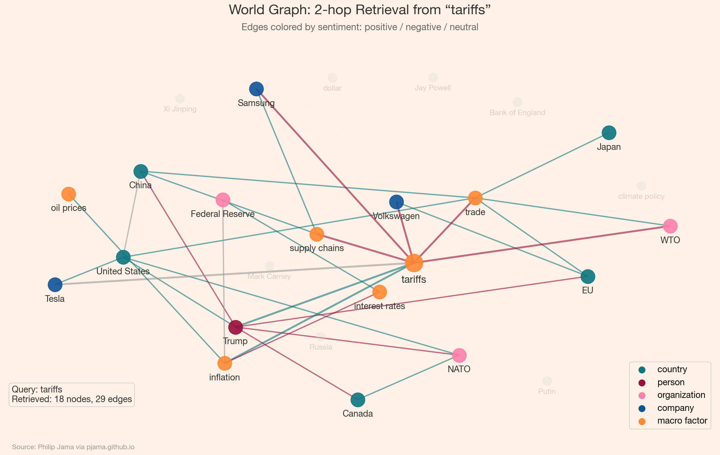
The retrieved subgraph around "tariffs" pulls in trade partners, affected companies, and inflationary consequences -- context that a flat vector search over article chunks would struggle to assemble coherently. Edge sentiment (green for positive, red for negative) adds a dimension that pure text retrieval cannot represent.

The Retrieval Pipeline

A GraphRAG system has four stages:

1. Graph construction -- build the knowledge graph from documents, using LLM extraction (Part 5 (LLM-Augmented Knowledge Graphs)), NLP pipelines, or structured data imports.
2. Query anchoring -- map the user's question to one or more seed nodes via entity linking, keyword matching, or embedding similarity.
3. Subgraph retrieval -- expand from seed nodes using a traversal strategy (k-hop, random walk, Personalized PageRank) to collect relevant context.
4. Context serialization -- convert the retrieved subgraph into a text prompt (node lists, triple lists, or natural-language summaries) and pass it to the LLM for generation.

Beyond k-Hop: Distance-Based Retrieval Metrics

The simple k-hop neighborhood used above retrieves every node within a fixed number of edges. This works for small, uniform graphs but becomes noisy on real knowledge graphs where some 2-hop neighbors are highly relevant and others are incidental. More sophisticated distance metrics produce tighter, higher-quality subgraphs.

Personalized PageRank

Instead of a hard hop cutoff, Personalized PageRank (PPR) runs a random walk that restarts at the query node with probability alpha. Nodes visited frequently by the walk receive high scores regardless of their exact hop distance. This naturally favors well-connected, structurally central neighbors over peripheral ones -- a node 3 hops away through a dense cluster may score higher than a 1-hop neighbor on a dead-end branch. PPR is the retrieval backbone of several production GraphRAG systems.

Embedding-Based Distance

When nodes carry vector embeddings (from an LLM, a GNN, or a knowledge graph embedding model like TransE), retrieval can combine graph distance with embedding similarity. A common approach scores candidate nodes as a weighted blend of shortest-path distance and cosine similarity to the query embedding. This captures both topological proximity and semantic relevance -- two nodes far apart in the graph but close in meaning (synonyms, paraphrases) still get retrieved.

Resistance Distance and Effective Conductance

The resistance distance from Part 3 also applies here: it measures connectivity between two nodes accounting for all paths, not just the shortest. In retrieval terms, a node connected to the query through many redundant paths is more "reachable" than one connected by a single fragile edge. Ranking by effective conductance (the inverse of resistance distance) naturally weights robustly connected neighbors higher. For an applied example, see the Organizational Network Analysis ↗ project, which uses resistance distance to surface connection recommendations from calendar data.

The Open-Source Landscape

Building GraphRAG from scratch clarifies the mechanics, but production systems typically rely on open-source frameworks that handle the plumbing. The ecosystem is maturing quickly.

LangChain GraphRetriever

LangChain's graph_rag integration provides a GraphRetriever that combines unstructured vector similarity search with structured metadata traversal. The key insight is that document metadata (tags, categories, source references) already forms a graph -- edges are defined by shared metadata fields. The retriever starts with a semantic search to find seed documents, then traverses metadata relationships to pull in structurally connected context. It supports pluggable vector stores (AstraDB, Cassandra, OpenSearch, Chroma) and offers built-in traversal strategies -- an eager strategy that expands to all neighbors within a depth limit, and MMR (Maximal Marginal Relevance) that balances relevance with diversity.

Microsoft GraphRAG

Microsoft's GraphRAG is an end-to-end pipeline that uses LLM extraction to build a knowledge graph, detects communities via Leiden clustering ↗, generates community summaries, and retrieves at multiple levels of abstraction -- local (entity neighborhoods) and global (community summaries). The global retrieval mode is distinctive: rather than traversing from a seed node, it queries pre-computed community summaries, enabling the system to answer broad questions ("What are the main themes in this corpus?") that entity-level retrieval cannot address.

Other Frameworks

• LlamaIndex Knowledge Graph Index: Builds a triple store from documents and supports both keyword and embedding-based entity retrieval with configurable traversal depth.
• Neo4j + LangChain: For teams already using Neo4j, LangChain provides a Neo4jGraph integration that translates natural-language questions into Cypher queries, combining the flexibility of a graph database with LLM-powered query generation.

The common pattern across all these frameworks is hybrid retrieval: vector search for semantic matching, graph traversal for structural context. The frameworks differ in how they construct the graph, what traversal strategies they offer, and how they serialize the retrieved subgraph into LLM context.

When to Use GraphRAG vs. Vector Search

GraphRAG shines when answers require multi-hop reasoning, when entity relationships matter, or when the knowledge base has rich relational structure. Vector search is simpler, faster, and sufficient when questions map directly to text passages. In practice, hybrid approaches -- vector retrieval for initial candidates, graph traversal for context expansion -- often outperform either alone.