Part 2 (Bayesian Sample Efficiency) introduced the idea that Bayesian methods support adaptive designs and early stopping. This article formalizes that idea. In practice, experimenters do not wait passively for a fixed sample size: they monitor dashboards, check interim results, and face pressure to call experiments early. The question is how to do this without destroying the validity of the conclusion.
Sequential testing provides the answer. Instead of committing to a single analysis at a predetermined endpoint, sequential methods define rules for evaluating evidence at multiple checkpoints throughout the experiment. Done correctly, these rules control error rates (frequentist) or provide calibrated posterior summaries (Bayesian) at every look.
The Peeking Problem
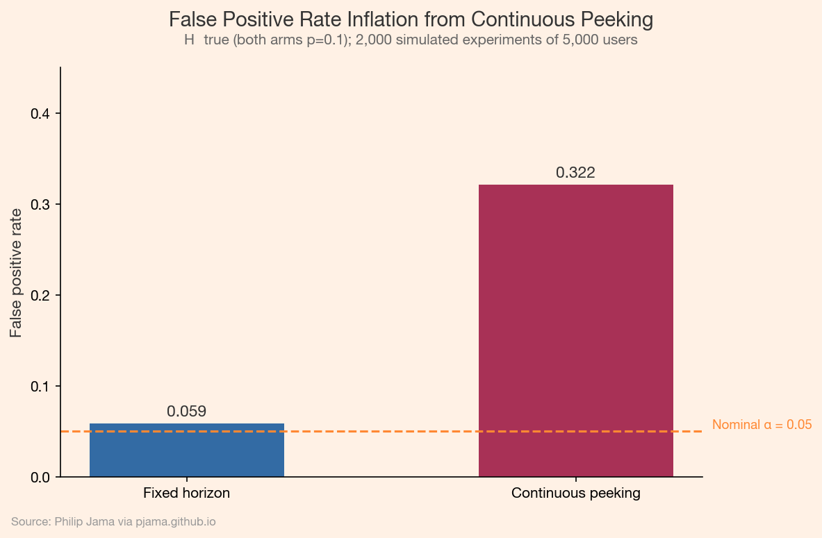
In a standard frequentist A/B test, the significance level alpha = 0.05 controls the false positive rate under a specific contract: you analyze the data exactly once, at the pre-specified sample size. If you check the p-value after every batch of users and stop as soon as p < 0.05, the true false positive rate inflates well beyond 5%. With continuous monitoring, it can exceed 25%.
The mechanism is straightforward. Under the null hypothesis, the test statistic follows a random walk. Given enough looks, even a random walk will cross any fixed threshold. Each peek is an additional opportunity for a false alarm. The more you peek, the more likely you are to see a "significant" result that is pure noise.
False positive rate inflation from continuous peeking compared to fixed-horizon analysis Show Python source
Group sequential designs are the frequentist solution to the peeking problem. They pre-specify a set of interim analyses (e.g., at 25%, 50%, 75%, and 100% of the target sample) and adjust the significance threshold at each look so that the overall Type I error rate stays at alpha.
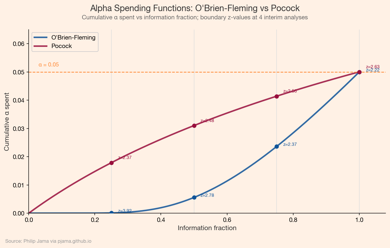
Alpha Spending Functions
An alpha spending functionalpha(t) maps the fraction of information collected t to the cumulative Type I error "spent" by that point. Two common choices:
O'Brien-Fleming: spends almost no alpha early and most at the final analysis. The early boundaries are stringent, making it hard to stop early unless the effect is large. The final-analysis threshold is close to the standard alpha = 0.05.
Pocock: spends alpha uniformly across looks. The boundaries are roughly equal at each interim analysis, making early stopping easier but the final threshold slightly more conservative.
The Lan-DeMets approach generalizes this: you specify the spending function up front, but the timing and number of looks can be chosen adaptively.
O'Brien-Fleming and Pocock alpha spending functions with boundary annotations Show Python source
import math
import matplotlib
matplotlib.use('Agg')
import matplotlib.pyplot as plt

FT_BG = '#FFF1E5'
FT_CLARET = '#990F3D'
FT_OXFORD = '#0F5499'
FT_TEAL = '#0D7680'
FT_MANDARIN = '#FF8833'

plt.rcParams.update({
    'figure.facecolor': FT_BG,
    'axes.facecolor': FT_BG,
    'savefig.facecolor': FT_BG,
    'font.family': 'sans-serif',
    'font.sans-serif': ['Helvetica Neue', 'Arial', 'sans-serif'],
    'axes.spines.top': False,
    'axes.spines.right': False,
})

def normal_cdf(z):
    if z < 0:
        return 1 - normal_cdf(-z)
    t = 1 / (1 + 0.2316419 * z)
    poly = t * (0.319381530 + t * (-0.356563782 + t * (
        1.781477937 + t * (-1.821255978 + t * 1.330274429))))
    return 1 - (1 / math.sqrt(2 * math.pi)) * math.exp(-0.5 * z * z) * poly

def normal_ppf(p):
    # Rational approximation for inverse normal CDF (Beasley-Springer-Moro)
    if p <= 0.5:
        return -normal_ppf(1 - p)
    t = math.sqrt(-2 * math.log(1 - p))
    c0, c1, c2 = 2.515517, 0.802853, 0.010328
    d1, d2, d3 = 1.432788, 0.189269, 0.001308
    return t - (c0 + c1 * t + c2 * t * t) / (1 + d1 * t + d2 * t * t + d3 * t * t * t)

alpha = 0.05
z_alpha2 = normal_ppf(1 - alpha / 2)

# Spending functions
ts = [i / 500 for i in range(1, 501)]

def obf_spending(t):
    return 2 - 2 * normal_cdf(z_alpha2 / math.sqrt(t))

def pocock_spending(t):
    return alpha * math.log(1 + (math.e - 1) * t)

obf = [obf_spending(t) for t in ts]
poc = [pocock_spending(t) for t in ts]

# Boundary z-values at 4 interim analyses
interims = [0.25, 0.50, 0.75, 1.0]
obf_increments = []
poc_increments = []
prev_obf = 0
prev_poc = 0
for t in interims:
    curr_obf = obf_spending(t)
    curr_poc = pocock_spending(t)
    obf_increments.append(curr_obf - prev_obf)
    poc_increments.append(curr_poc - prev_poc)
    prev_obf = curr_obf
    prev_poc = curr_poc

obf_z = [normal_ppf(1 - inc / 2) if inc > 0 else float('inf') for inc in obf_increments]
poc_z = [normal_ppf(1 - inc / 2) if inc > 0 else float('inf') for inc in poc_increments]

fig, ax = plt.subplots(figsize=(9, 5.5))

ax.plot(ts, obf, color=FT_OXFORD, linewidth=2.5, label="O'Brien-Fleming", alpha=0.85)
ax.plot(ts, poc, color=FT_CLARET, linewidth=2.5, label='Pocock', alpha=0.85)
ax.axhline(y=alpha, color=FT_MANDARIN, linewidth=1.2, linestyle='--')
ax.text(0.03, alpha + 0.002, f'\u03b1 = {alpha}', fontsize=9, color=FT_MANDARIN)

# Mark interim analyses
for i, t in enumerate(interims):
    ax.axvline(x=t, color='#dddddd', linewidth=0.8, zorder=1)
    obf_val = obf_spending(t)
    poc_val = pocock_spending(t)
    ax.plot(t, obf_val, 'o', color=FT_OXFORD, markersize=6, zorder=4)
    ax.plot(t, poc_val, 'o', color=FT_CLARET, markersize=6, zorder=4)
    ax.text(t + 0.02, obf_val, f'z={obf_z[i]:.2f}', fontsize=7.5, color=FT_OXFORD, va='bottom')
    ax.text(t + 0.02, poc_val + 0.001, f'z={poc_z[i]:.2f}', fontsize=7.5, color=FT_CLARET, va='bottom')

ax.set_xlim(0, 1.08)
ax.set_ylim(0, alpha * 1.3)
ax.set_xlabel('Information fraction', fontsize=11, color='#333333')
ax.set_ylabel('Cumulative \u03b1 spent', fontsize=11, color='#333333')
ax.legend(fontsize=10, framealpha=0.9, loc='upper left')

fig.text(0.5, 0.97, "Alpha Spending Functions: O'Brien-Fleming vs Pocock",
         ha='center', fontsize=14, fontweight='bold', color='#333333')
fig.text(0.5, 0.935, 'Cumulative \u03b1 spent vs information fraction; boundary z-values at 4 interim analyses',
         ha='center', fontsize=10, color='#666666')
fig.text(0.02, 0.01, 'Source: Philip Jama via pjama.github.io',
         fontsize=8, color='#999999', ha='left')
fig.tight_layout(rect=[0, 0.03, 1, 0.92])
fig.savefig('spending_functions.png', dpi=150, bbox_inches='tight')

print('wrote spending_functions.png')
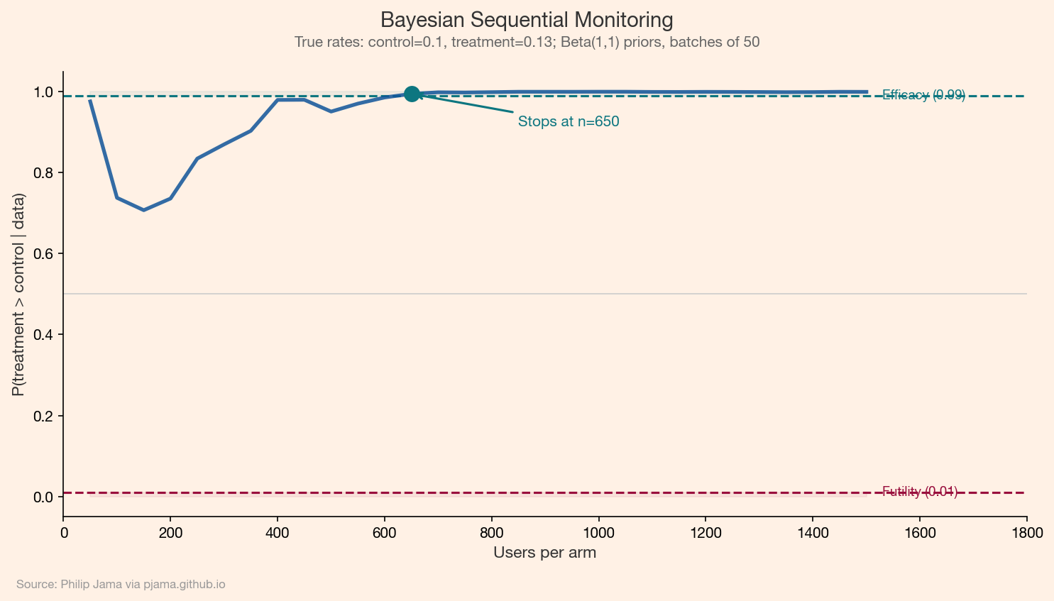
Bayesian Sequential Monitoring
The Bayesian approach to sequential analysis avoids the peeking problem by construction. The posterior is always valid: it represents a coherent summary of the evidence seen so far, regardless of how many times you look at it. There is no need to adjust for multiple looks because the posterior does not make a promise about long-run error rates that peeking could violate.
The standard Bayesian monitoring procedure tracks the posterior probability that treatment beats control (P(p_T > p_C | data)) at each interim analysis. Decisions follow threshold rules:
Stop for efficacy: if P(p_T > p_C | data) > theta_upper (e.g., 0.99), declare the treatment a winner.
Stop for futility: if P(p_T > p_C | data) < theta_lower (e.g., 0.01), declare no meaningful effect.
Continue: otherwise, collect more data.
The thresholds theta_upper and theta_lower are design parameters. More aggressive thresholds (0.95/0.05) stop experiments sooner but increase the chance of incorrect decisions. Conservative thresholds (0.99/0.01) require more data but provide stronger evidence.
Posterior probability of treatment superiority over time with stopping boundaries Show Python source
Group sequential (frequentist): controls the probability of a false positive across all possible stopping points. The guarantee is about long-run error rates under repeated use.
Bayesian sequential: reports the probability of a correct decision given the data actually observed. The guarantee is about the coherence of the current inference.
In practice, the operating characteristics (how often each method stops early, expected sample size, error rates) are often similar when calibrated to comparable decision thresholds. The philosophical difference matters most when communicating results: "we stopped because the posterior probability exceeded 0.99" is more intuitive to most stakeholders than "we stopped because the z-statistic crossed the O'Brien-Fleming boundary."
Stopping for Futility
Most discussions of early stopping focus on efficacy: detecting a winner quickly. Futility stopping is equally valuable. If the treatment effect is negligibly small, continuing the experiment wastes traffic and delays the next test.
A Bayesian futility rule stops when the posterior probability that the treatment effect exceeds a minimum detectable effect (MDE) is below some threshold. For example: stop if P(delta > MDE | data) < 0.05, where delta = p_T - p_C. This is more useful than simply checking whether the posterior favors treatment, because a tiny positive effect that will never be practically meaningful is not worth chasing.
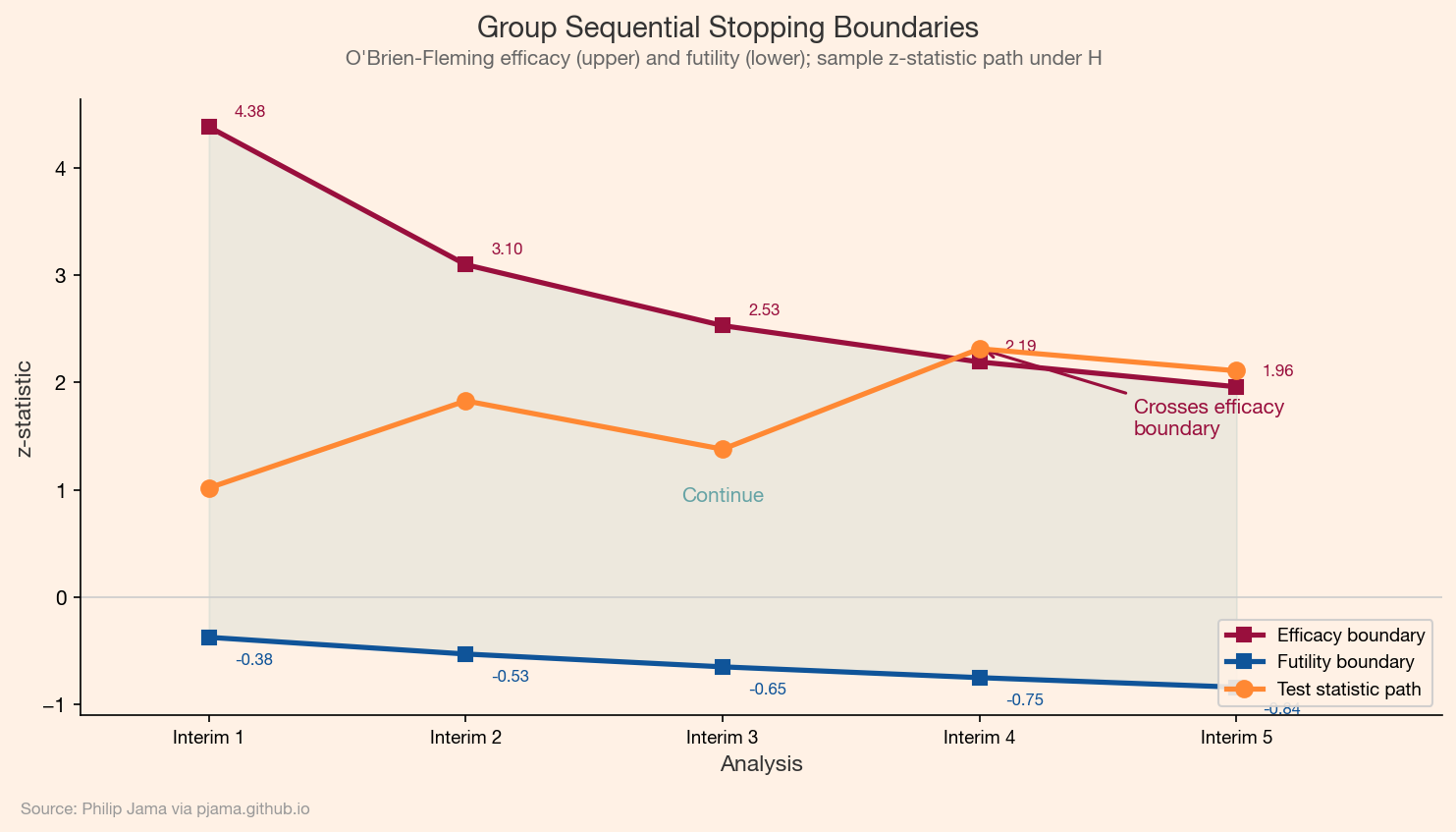
Stopping Boundaries
The following simulation visualizes both efficacy and futility boundaries on a single plot. The test statistic (or posterior summary) traces a path through the monitoring region. When it crosses an upper boundary, the experiment stops for efficacy. When it crosses a lower boundary, it stops for futility. The region between the boundaries is the continuation zone.
Efficacy and futility stopping boundaries with a sample test statistic path Show Python source
import math
import random
import matplotlib
matplotlib.use('Agg')
import matplotlib.pyplot as plt

random.seed(3)

FT_BG = '#FFF1E5'
FT_CLARET = '#990F3D'
FT_OXFORD = '#0F5499'
FT_TEAL = '#0D7680'
FT_MANDARIN = '#FF8833'

plt.rcParams.update({
    'figure.facecolor': FT_BG,
    'axes.facecolor': FT_BG,
    'savefig.facecolor': FT_BG,
    'font.family': 'sans-serif',
    'font.sans-serif': ['Helvetica Neue', 'Arial', 'sans-serif'],
    'axes.spines.top': False,
    'axes.spines.right': False,
})

def normal_ppf(p):
    if p <= 0.5:
        return -normal_ppf(1 - p)
    t = math.sqrt(-2 * math.log(1 - p))
    c0, c1, c2 = 2.515517, 0.802853, 0.010328
    d1, d2, d3 = 1.432788, 0.189269, 0.001308
    return t - (c0 + c1 * t + c2 * t * t) / (1 + d1 * t + d2 * t * t + d3 * t * t * t)

K = 5
interims = list(range(1, K + 1))
info_fracs = [k / K for k in interims]

z_alpha2 = normal_ppf(0.975)

# O'Brien-Fleming-style efficacy boundary
upper = [z_alpha2 / math.sqrt(t) for t in info_fracs]

# Futility boundary (beta-spending style)
z_beta = normal_ppf(0.80)
lower = [-z_beta * math.sqrt(t) for t in info_fracs]

# Simulate z-statistic path under H1 with drift
drift = 2.2
z_path = []
for k in range(1, K + 1):
    t = k / K
    z = drift * math.sqrt(t) + random.gauss(0, 0.35)
    z_path.append(z)

# Find crossing point
cross_interim = None
for i in range(K):
    if z_path[i] >= upper[i]:
        cross_interim = i
        break
    if z_path[i] <= lower[i]:
        cross_interim = i
        break

fig, ax = plt.subplots(figsize=(10, 5.5))

# Shade continuation region
ax.fill_between(interims, lower, upper, color=FT_TEAL, alpha=0.07, zorder=1)

# Boundaries
ax.plot(interims, upper, color=FT_CLARET, linewidth=2.5, marker='s', markersize=7,
        label='Efficacy boundary', zorder=3)
ax.plot(interims, lower, color=FT_OXFORD, linewidth=2.5, marker='s', markersize=7,
        label='Futility boundary', zorder=3)

# Sample path
ax.plot(interims, z_path, color=FT_MANDARIN, linewidth=2.5, marker='o', markersize=8,
        label='Test statistic path', zorder=4)

ax.axhline(y=0, color='#cccccc', linewidth=0.8)

# Annotate crossing
if cross_interim is not None:
    cx = interims[cross_interim]
    cy = z_path[cross_interim]
    ax.annotate('Crosses efficacy\nboundary', xy=(cx, cy),
                xytext=(cx + 0.6, cy - 0.8),
                fontsize=10, color=FT_CLARET, fontweight='bold',
                arrowprops=dict(arrowstyle='->', color=FT_CLARET, lw=1.5),
                ha='left')

# Label boundary values
for i in range(K):
    ax.text(interims[i] + 0.1, upper[i] + 0.1, f'{upper[i]:.2f}',
            fontsize=8, color=FT_CLARET)
    ax.text(interims[i] + 0.1, lower[i] - 0.25, f'{lower[i]:.2f}',
            fontsize=8, color=FT_OXFORD)

ax.set_xlim(0.5, K + 0.8)
ax.set_xticks(interims)
ax.set_xticklabels([f'Interim {k}' for k in interims], fontsize=9)
ax.set_xlabel('Analysis', fontsize=11, color='#333333')
ax.set_ylabel('z-statistic', fontsize=11, color='#333333')
ax.legend(fontsize=9, framealpha=0.9, loc='lower right')

# Add continuation region label
mid_interim = interims[K // 2]
mid_y = (upper[K // 2] + lower[K // 2]) / 2
ax.text(mid_interim, mid_y, 'Continue', fontsize=10, color=FT_TEAL,
        ha='center', va='center', alpha=0.6, fontstyle='italic')

fig.text(0.5, 0.97, 'Group Sequential Stopping Boundaries',
         ha='center', fontsize=14, fontweight='bold', color='#333333')
fig.text(0.5, 0.935, "O'Brien-Fleming efficacy (upper) and futility (lower); sample z-statistic path under H\u2081",
         ha='center', fontsize=10, color='#666666')
fig.text(0.02, 0.01, 'Source: Philip Jama via pjama.github.io',
         fontsize=8, color='#999999', ha='left')
fig.tight_layout(rect=[0, 0.03, 1, 0.92])
fig.savefig('stopping_boundaries.png', dpi=150, bbox_inches='tight')

print('wrote stopping_boundaries.png')
Practical Guidance
Sequential testing in production requires discipline:
Pre-register the monitoring schedule. Decide how many interim looks, at what information fractions, and with what thresholds before the experiment starts. Ad hoc decisions after seeing data undermine the guarantees.
Automate the monitoring. Manual dashboard checks invite unplanned peeks. Build the sequential analysis into the experiment platform so that boundary crossings trigger alerts rather than relying on human judgment about when to look.
Account for delayed outcomes. If the primary metric takes days to mature (e.g., 7-day retention), interim analyses based on incomplete outcome data will be biased toward zero. Use the outcome window appropriate for the metric, not the most recent data.
Report the stopping rule with the result. A sequential experiment that stopped early at interim look 3 of 5 carries different interpretive weight than a fixed-horizon analysis. Transparency about the design supports reproducibility.
Connection to the Series
Sequential testing completes a loop that began in Part 1 (Online Experiments with a Bayesian Lens). The Beta posteriors from that article update continuously as data arrives. Part 2 (Bayesian Sample Efficiency) showed that this updating can reduce the required sample size. This article provides the formal rules for acting on that updating: when the posterior crosses a boundary, you stop.
Part 4 (Multi-Armed Bandits and Thompson Sampling) took a different approach to the same tension: rather than deciding when to stop, Thompson sampling decides how to allocate at each round. And Part 5 (Causal Inference from Observational Data) addressed what to do when you cannot run the experiment at all. Together, the six articles in this series cover the full lifecycle of evidence-based decisions: from designing experiments and analyzing posteriors, through adaptive allocation and observational inference, to the formal rules for stopping and committing.
Sequential monitoring decides when to stop an experiment, but the explore-exploit tradeoff from bandit allocation and the observational methods from causal inference each address different gaps in the decision pipeline.