Articles /Network Graph Analysis /Part 9
Causal and Bayesian Networks
DAGs, interventions, and counterfactual reasoning on graphs
Causal InferenceBayesian NetworksDAGDo-CalculusCounterfactualsPythonProbabilistic Graphical Models
Articles /Network Graph Analysis /Part 9
Causal InferenceBayesian NetworksDAGDo-CalculusCounterfactualsPythonProbabilistic Graphical Models
Temporal models capture when connections change but not why. Causal and Bayesian networks use directed acyclic graphs to encode cause-and-effect, turning the graph from a descriptive tool into a reasoning engine. Where Part 8 (Temporal Graphs) modeled evolving structure, this final article asks what that structure means: which edges represent genuine causal influence, and what would happen if we intervened on a node.
The framework comes from Judea Pearl’s causal inference tradition, and one running example will carry it through the article: a microservices outage. Service A (an API gateway) calls Service B (authentication) and Service C (product catalog); C calls Service D (the database layer). Distributed tracing timestamps every call, and one afternoon end-to-end latency spikes. Which service is the root cause? We start with the DAG as a causal model, develop the do-calculus for reasoning about interventions, add Bayesian networks for probabilistic inference, and close with counterfactual reasoning: the strongest claim a graph can support.
In a causal DAG, nodes represent variables and directed edges represent direct causal effects. The absence of an edge is an assertion: it claims one variable does not directly cause another. Note which way the arrows run in the incident graph: A calls C, and C calls D, but latency propagates from D through C to A. The causal DAG is the reversed call graph, with an edge from each service to the services that wait on it.
Three structures organize everything that follows. A confounder is a common cause of two variables. Shared infrastructure (a saturated load balancer, a noisy neighbor on the same host) raises latency in Service B and in the user-facing total at the same time, so the two move together even if B causes nothing downstream. A mediator lies on the causal path: Service D’s slow queries reach the user through Service C, which waits on them. A collider is a common effect of two variables. If high latency and elevated error rates each independently trigger paging, then among paged incidents latency and error rate are spuriously anti-correlated: the pages with modest latency tend to be the ones with severe errors. Conditioning on a collider (studying only paged incidents) manufactures an association that does not exist in the system, the same mechanism as Berkson’s paradox.
Each structure demands different treatment. Confounders must be adjusted for, mediators define indirect effects, and colliders must not be conditioned on. The DAG makes these requirements explicit and testable.
These three structures determine what a DAG can tell you about conditional independence, a property called d-separation. Trace every path between two variables and check whether each is blocked by the conditioning set: conditioning on a confounder blocks the spurious path, conditioning on a collider opens one. If Service B and user-facing latency are d-separated given the shared-infrastructure metrics, every association between them is confounding, a fact the root cause analysis below will use. This is why the observational causal inference article emphasized drawing the DAG before choosing which variables to adjust for: the graph’s structure dictates what to condition on, and getting it wrong introduces bias rather than removing it.
D-separation also gives the DAG testable implications. Every independence it predicts can be checked against the trace data. If Service B’s latency still correlates with the user-facing total after conditioning on infrastructure metrics, the DAG is missing an edge; structure learning algorithms, covered below, exploit exactly this to discover causal graphs from data.
Observational data tells us $P(Y \mid X = x)$, the probability of $Y$ given that we observe $X$ taking value $x$. The causal question is different: $P(Y \mid \text{do}(X = x))$, the probability of $Y$ if we set $X$ to $x$ by intervention. Pearl’s do-operator formalizes the distinction through graphical surgery: to compute the effect of $\text{do}(X = x)$, delete all incoming edges to $X$ in the DAG (since the intervention overrides whatever would have caused $X$) and compute the resulting distribution. The difference is concrete in the incident graph. Observing that Service D is slow raises the probability that everything else is slow too, because slowness is evidence of shared load. Forcing D to its baseline with a cache flush is do(D = normal): it severs D from its usual causes, and whatever latency remains is not D’s doing.
The key question is when we can compute this interventional distribution from observational data alone. The backdoor criterion provides the most common answer. Some paths between treatment and outcome carry the causal effect (they flow forward through direct or mediated connections). Others are confounding paths: they flow from a common cause into both treatment and outcome, creating a spurious association. If we can find a set of variables $Z$ that blocks all confounding paths, opens no collider paths, and contains no descendants of the treatment, the causal effect reduces to a conditional probability weighted over $Z$:
$$P(Y \mid \text{do}(X = x)) = \sum_z P(Y \mid X = x, Z = z) \; P(Z = z)$$
In the incident graph, $Z$ is the shared-infrastructure metrics: condition on them, and the observational traces identify the causal effect of any service on user-facing latency. The front-door criterion covers the opposite bind, where the confounder is unmeasured but an observed mediator carries the entire effect. Pearl’s canonical case is smoking and cancer confounded by an unmeasured genotype: tar deposits mediate the effect, so chaining the smoking-to-tar and tar-to-cancer estimates recovers what the missing confounder would otherwise block. The next figure shows the graphical surgery on the incident graph.
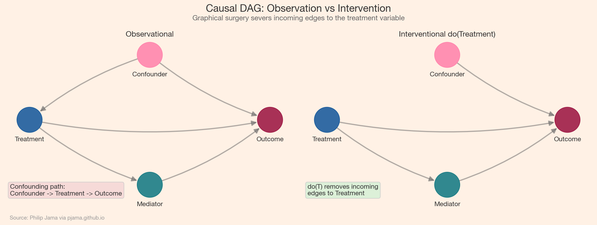
Randomized experiments implement the do-operator physically. When we randomly assign subjects to treatment or control, we sever the connection between the treatment variable and any confounders: exactly the graphical surgery that do(X = x) performs on the DAG. This is why randomization eliminates confounding bias without requiring us to identify or measure confounders.
The Online Experiments with a Bayesian Lens article analyzed A/B tests from this perspective: random assignment guarantees that the backdoor criterion is satisfied with $Z = \varnothing$, so the observed difference in outcomes is the causal effect. When randomization is impossible (in observational studies, natural experiments, or retrospective analyses), the do-calculus provides the machinery for determining whether and how the causal effect can still be recovered.
A caution before the next tool: the DAGs so far have been causal, but the same formalism has a second, purely statistical use, and conflating the two is the classic mistake in this field. A Bayesian network pairs a DAG with a set of conditional probability distributions (CPDs): each node has a distribution conditioned on its parents, and together these local specifications define the joint distribution through the factorization property: $P(X_1, \ldots, X_n) = \prod_i P(X_i \mid \text{Parents}(X_i))$. Nothing in that definition requires the arrows to be causal. Many different DAGs can encode the same joint distribution, and a Bayesian network is a valid compression of the data under any of them; reading its arrows as cause-and-effect is an additional assumption, exactly the assumption the structure-learning section below interrogates. The factorization is still enormously useful: it exploits conditional independence to represent a large joint distribution compactly and to answer probabilistic queries efficiently.
The classic textbook example uses three variables: Rain, Sprinkler, and Grass Wet. Rain influences both the sprinkler (negatively: you turn off the sprinkler when it rains) and whether the grass is wet. The sprinkler also affects whether the grass is wet. Given the observation that the grass is wet, we want the posterior probability that it rained: a computation that requires combining the prior on rain with the likelihoods through each causal pathway.
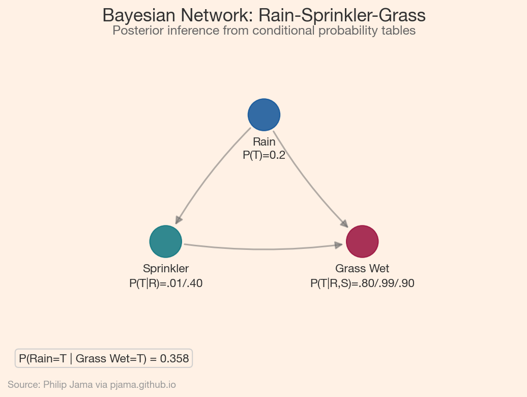
Inference in a Bayesian network means computing posteriors given evidence, and the graph’s structure sets the cost. Tree-like graphs admit fast exact inference through variable elimination; richly interconnected graphs force approximation (MCMC sampling, variational methods) even when each node has few neighbors.
In practice, the causal DAG is rarely known with certainty. Structure learning algorithms attempt to recover the graph from data. The fundamental limitation is that observational data alone cannot distinguish between DAGs that encode the same set of conditional independencies. Such DAGs form a Markov equivalence class: they share the same skeleton (the same edges, ignoring direction) and the same v-structures (colliders), and no observational test can tell them apart. Structure learning can narrow the possibilities to this class but cannot pinpoint the unique causal DAG without additional assumptions or experimental data.
Two families of algorithms dominate. Constraint-based methods like the PC algorithm test conditional independencies in the data, remove edges between independent variables, and orient the remaining edges using structural patterns (e.g., if two non-adjacent nodes both point to a third, that collision pattern reveals edge direction). Score-based methods like greedy equivalence search (GES) search over graph structures to optimize a fit-complexity tradeoff, typically using the Bayesian Information Criterion. Hybrid approaches combine both strategies. In practice, tooling matters less than workflow: pgmpy, CausalNex, and DoWhy cover structure learning, inference, and effect estimation between them, and purely data-driven learning is only a starting point. Domain experts fix the edges they know (temporal ordering, established mechanisms) and let the algorithm fill in the uncertain relationships.
Pearl’s causal ladder distinguishes three levels of reasoning, each strictly more powerful than the last. Association (level 1) asks "what is": given that Service A is slow, how likely is Service D to be slow? This is standard observational correlation. Intervention (level 2) asks "what if we do": if we force Service D’s latency to its baseline (do(D = normal)), does user-facing latency recover? This requires the do-calculus machinery developed above. Counterfactual (level 3) asks "what if things had been different": given that the outage did occur, would it have occurred if Service D had not exceeded its memory limit?
Counterfactual reasoning follows a three-step procedure. First, abduction: use the observed evidence (all measured latencies during the incident) to infer the values of unobserved variables (network congestion, background load). Second, action: modify the DAG to reflect the hypothetical intervention (set Service D’s memory usage to normal). Third, prediction: propagate forward through the modified DAG to compute the counterfactual outcome. The result is an attribution score: the probability that the outage would not have occurred in the counterfactual world.
D-separation provides the first filter. If Service B and user-facing latency are d-separated given the shared-infrastructure metrics (load-balancer saturation, host CPU), then B’s correlation with the outage is confounding rather than causation, and B drops out of the candidate set. The cleanest case is an asynchronous call the gateway never waits on: then no causal path from B to user-facing latency exists at all. This narrows the candidate set without any statistical estimation, using only the graph structure.
For the remaining candidates, the do-calculus formalizes the root cause question. The interventional query P(user_latency > threshold | do(C = normal)) asks: if we could reset Service C’s latency, how much would user-facing latency improve? If the backdoor criterion is satisfied (by conditioning on shared infrastructure metrics), this quantity can be estimated from the observational traces without actually intervening on the running system.
The counterfactual step completes the analysis. After the incident, the post-mortem asks: "Would the outage have occurred if Service D had not exceeded its memory limit?" The three-step procedure (abduct the hidden variables from the incident data, impose do(D_memory = normal), predict the resulting latencies) produces a probability. If it is low, Service D’s memory spike was the root cause. If it is high, the outage would have happened anyway, and the true cause lies elsewhere in the graph.
The code below runs the full procedure on a simulated incident: abduct the exogenous conditions from the observed telemetry, apply each candidate fix as an intervention, and compute the probability that user-facing latency would have cleared its SLO.
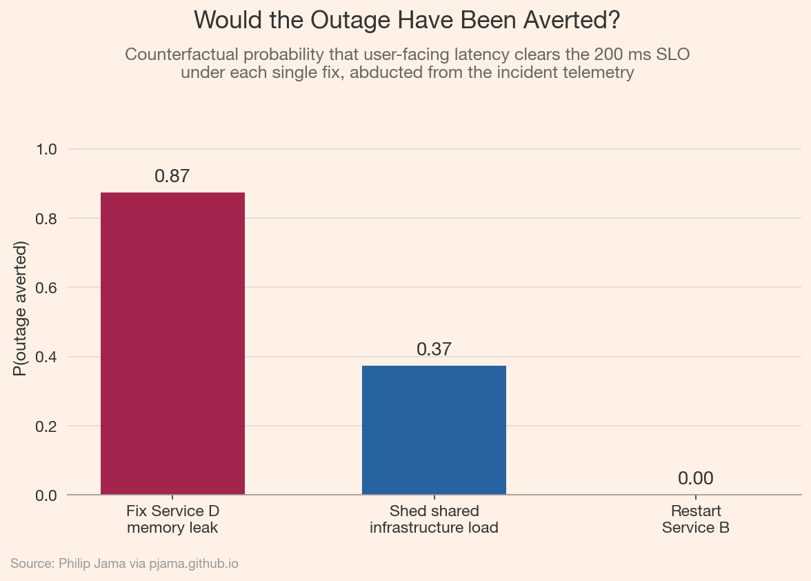
This layered approach (association for monitoring, intervention for diagnosis, counterfactual for attribution) mirrors how incident response teams actually reason. The causal graph formalizes each step and makes the assumptions explicit. When those assumptions are encoded in a DAG, they become auditable: anyone can inspect the graph, check the d-separation claims, and challenge the causal model.
Nothing in the ladder is specific to microservices. The geopolitical world graph from Part 6 (GraphRAG) supports the same three levels. Association is monitoring: sanctions headlines co-occur with shipping-rate spikes. Intervention is scenario analysis: what happens to freight rates and gold under do(strait = closed), holding the graph’s other mechanisms fixed? Counterfactual is attribution: given that gold did spike, would it have spiked had the strait stayed open, or was the move already in motion from rate expectations? These questions are harder than in a service mesh because the DAG is contested and confounding is everywhere, which is exactly why an explicit graph matters: the assumptions become visible and debatable. The World Graph runs this reasoning on daily news, encoding causal mechanisms between actors, assets, and events and surfacing the scenarios most likely to unfold.
This series has moved through progressively stronger claims about what graphs can tell us. Part 1 (Foundations) defined the vocabulary: nodes, edges, paths, components. Subsequent articles measured structure (centrality, communities), extracted it from text (knowledge graphs), learned representations of it (GNNs), and tracked how it changes (temporal networks). Each step added analytical power while staying within the realm of association: describing patterns in data.
Causal and Bayesian networks cross that boundary. The DAG is no longer a summary of observed relationships but a claim about the data-generating process. D-separation produces testable predictions. The do-calculus turns observational data into interventional conclusions. Counterfactuals attribute specific outcomes to specific causes. The shift from association to causation is what separates description from understanding, and graphs are the language in which that shift is expressed.
The causal reasoning developed here connects directly to the Decision Science series: Bayesian A/B testing is intervention with randomization, observational causal inference is intervention without it, and the DAG framework unifies both.
If you're exploring related work and need hands-on help, I'm open to consulting and advisory. Get in touch›